7 Analysis of Covariance (ANCOVA)
In an ANOVA the interest lies in the differences among means. In a linear regression the interest lies in the intercept and slope parameters of regression lines, or perhaps other parameters of biological interest, e.g. asymptotic and effective doses (e.g, \(latex LD_{50}\) levels in the nonlinear case. The combination of ANOVA and regression is called Analysis of Covariance (ANCOVA). It is an underutilized method that makes sequential tests for testing various hypotheses. Usually it is confined to linear regressions but can be equally powerful when used in nonlinear relationships. However, in this section we only consider the linear ANCOVA.
7.1 Example 1: Mechanical Weed Control
A mechanical weed control experiment (Rasmussen et al. 2008] tested the effect of intensity of harrowing (1, 2, 3, or 4 times), either along or across the direction of sowing (factors) on the weed cover left after the harrowing.
Harrowing<- read.csv2("http://rstats4ag.org/data/Harrowing.csv")
head(Harrowing,3)
## plot leaf weeds int direction yield
## 1 1 0.18623052 103.33763 0 along 4.21
## 2 2 0.12696533 54.02022 1 along 4.08
## 3 3 0.09006582 23.44035 2 along 3.92Lets look at the relationships in Figure 7.1.
library(lattice)##
## Attaching package: 'lattice'## The following object is masked from 'package:drcData':
##
## barleyxyplot(weeds ~ int | direction, data = Harrowing,
ylab="Weed Cover",xlab="Intensity of Harrowing" ) 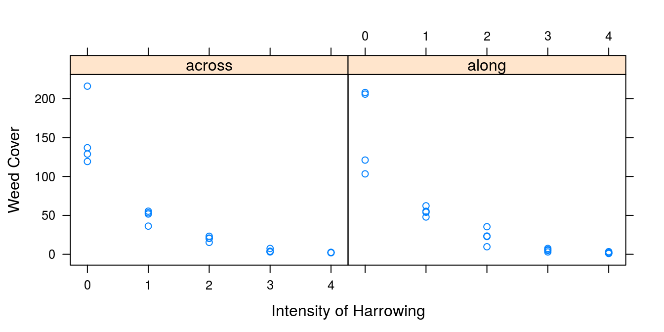
Figure 7.1: The relationship between weed cover and intensity of harrowing either across or along the direction of sowing.
The relationships above does not look very linear, it looks like an exponential decreasing leaf cover. If this assumption is correct we can make the relationship linear by taking the logarithm of weed cover.
xyplot(log(weeds) ~ int | direction, data = Harrowing,
       ylab="Log(Weed Cover)",xlab="Intensity of Harrowing",
       panel = function(x,y)
       {panel.xyplot(x,y)
        panel.lmline(x,y)})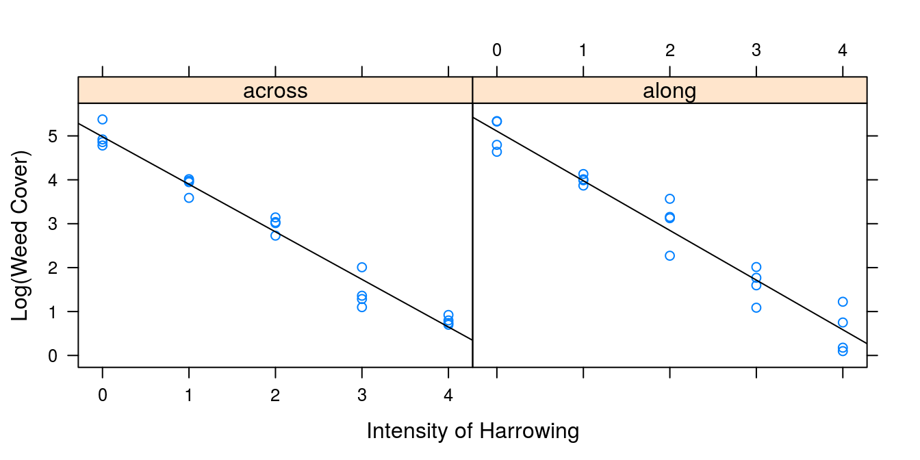
Figure 7.2: Same data as in 7.1 using the logarithm of weed cover (y-axis) gives a relationship that looks linear on the intensity of harrowing within the directions of harrowing.
Apparently, the assumption of a straight line relationship looks good, but we have to do statistics to substantiate this hypothesis. It is of interest to know whether the harrowing direction (across or along the rows) had the same effect on weed cover. Statistically, we want to know if the two regression lines are similar in term of regression slopes. This can be done by sequential testing:
- Ordinary ANOVA where
intis turned into a factorfactor(int) - ANCOVA with interaction; meaning that the regression lines can have both different slopes and intercepts
Harrowing$Log.weeds <- log(Harrowing$weeds)
m1 <- lm(Log.weeds ~ factor(int) * direction, data = Harrowing)
m2 <- lm(Log.weeds ~ int * direction, data = Harrowing)
anova(m1, m2)
## Analysis of Variance Table
##
## Model 1: Log.weeds ~ factor(int) * direction
## Model 2: Log.weeds ~ int * direction
## Res.Df RSS Df Sum of Sq F Pr(>F)
## 1 30 3.5350
## 2 36 4.2754 -6 -0.74048 1.0474 0.4152m1, an ordinary ANOVA, is the most general model with no assumption of any particular relationship. m2is the ANCOCVA, which assumes there is a linear relationship between harrowing direction and intensity. The int * direction in m2 means that there is an interaction between the slopes depending on the direction of harrowing. Or in other words the slopes of the regression lines are different. The test for lack of fit is not significant (p=0.42) so we can assume a linear relationship applies to the log-transformed response variable.
We can further refine the analysis through sequential testing: * Assuming similar slope but different intercept depending of direction of harrowing * Assuming that the directions of harrowing does not influence regression lines, e.i, similar line
To do this, we first test the regression model with an interaction term, m2, with a regression model where we assume no interaction,m3, which mean the slopes of the regression lines are similar:
m3 <- lm(Log.weeds ~ int + direction, data = Harrowing)
anova(m2,m3)
## Analysis of Variance Table
##
## Model 1: Log.weeds ~ int * direction
## Model 2: Log.weeds ~ int + direction
## Res.Df RSS Df Sum of Sq F Pr(>F)
## 1 36 4.2754
## 2 37 4.3207 -1 -0.045295 0.3814 0.5407The lack of fit test is again not significant so we can assume that there is no interaction, and conclude that the regression slopes are similar. The final test will determine whether the direction of harrowing influences the relationship between log(Weed Cover) and intensity of harrowing?
m4 <- lm(Log.weeds ~ int, data = Harrowing)
anova(m4, m3)
## Analysis of Variance Table
##
## Model 1: Log.weeds ~ int
## Model 2: Log.weeds ~ int + direction
## Res.Df RSS Df Sum of Sq F Pr(>F)
## 1 38 4.3311
## 2 37 4.3207 1 0.010344 0.0886 0.7677Again, no significance here either (p=0.77); so we end up from the most general model (ANOVA) to the most simple ANCOVA: direction of harrowing does not matter and the relationship between log(weeds)and intensity of harrowing is linear.
summary(m4)##
## Call:
## lm(formula = Log.weeds ~ int, data = Harrowing)
##
## Residuals:
## Min 1Q Median 3Q Max
## -0.63622 -0.25226 0.06307 0.28256 0.73686
##
## Coefficients:
## Estimate Std. Error t value Pr(>|t|)
## (Intercept) 5.04478 0.09246 54.56 <2e-16 ***
## int -1.10710 0.03775 -29.33 <2e-16 ***
## ---
## Signif. codes: 0 '***' 0.001 '**' 0.01 '*' 0.05 '.' 0.1 ' ' 1
##
## Residual standard error: 0.3376 on 38 degrees of freedom
## Multiple R-squared: 0.9577, Adjusted R-squared: 0.9566
## F-statistic: 860.3 on 1 and 38 DF, p-value: < 2.2e-16In order to illustrate the result we use the code below to create Figure 7.3. For illustration purposes we have separated the means into direction across and along even though it is not necessary.
library(dplyr)
Plot.means <- Harrowing %>%
  group_by(int, direction) %>%
  summarise(count = n(), Log.Weeds = mean(Log.weeds))

par(mgp=c(2,.7,0), mar=c(3.2,3.2,.5,.5))
plot(Log.Weeds~int, data = Plot.means, bty="l",
     pch = as.numeric(direction),
     xlab="Harrowing intensity",
     ylab="Log(weed cover)")
abline(m4)
legend("bottomleft", c("Across", "Along"), pch = c(2,1))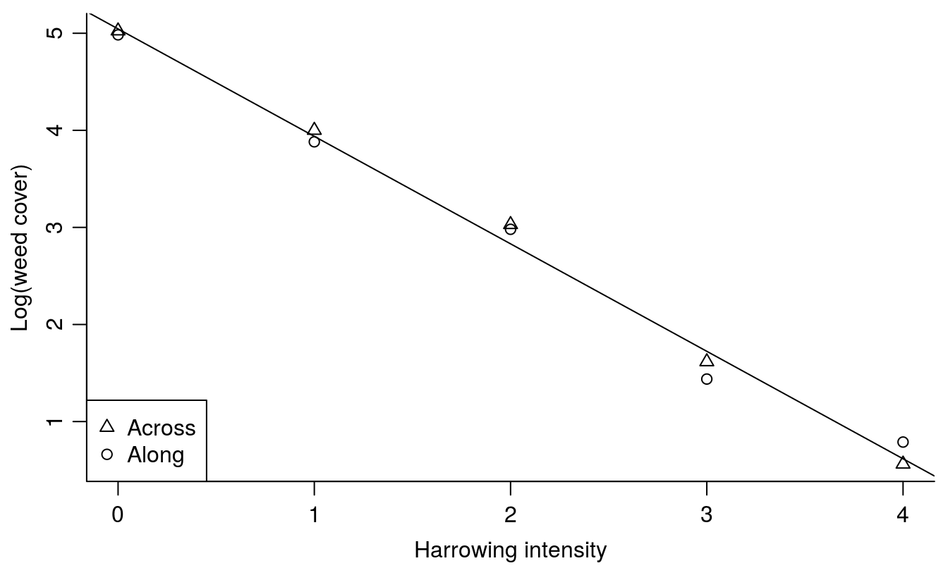
Figure 7.3: Summary plot of the harrowing experiments. There is no difference between the direction of harrowing and, therefore, only one regression line is necessary.
The slope is -1.11 (0.04) which means that with an increase in harrowing intensity the logarithm of weed cover decreases by -1.11. In fact the relationship is an exponential decay curve where the relative rate of change is exp(-1.11)= 0.3296 wherever we are on the curve.
7.2 Example 2: Duration of competition
In 2006 and 2007, field studies were conducted near Powell, Wyoming to determine the effects of Salvia reflexa (lanceleaf sage) interference with sugarbeet. This data was published in Odero et al. 2010. Salvia reflexa was seeded alongside the sugarbeet crop at a constant density, and allowed to compete for time periods ranging from 36 to 133 days after sugarbeet emergence. Yields (Yield_Mg.ha) were determined at the end of the season.
lanceleaf.sage<-read.csv("http://rstats4ag.org/data/lanceleafsage.csv")
head(lanceleaf.sage,n=3)
## Replicate Duration Year Yield_Mg.ha Yield.loss.pct
## 1 1 36 2006 67.26 98.05
## 2 1 50 2006 60.34 87.96
## 3 1 64 2006 53.69 78.27library(lattice)
xyplot(Yield_Mg.ha~Duration|factor(Year),data=lanceleaf.sage,
ylab= "Sugarbeet root yield (t/ha)",
xlab="Duration of competition from _Salvia reflexa_",
panel = function(x,y)
{panel.xyplot(x,y)
panel.lmline(x,y)})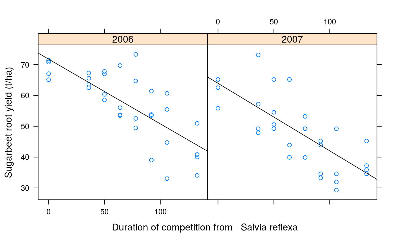
Figure 7.4: Duration of Salvia reflexa competition effect on yield of sugar beet in two years.
As was the case with the harrowing experiment we do sequential testing. First, we compare the ANCOVA with the most general model, an AVOVA:
lm1 <- lm(Yield_Mg.ha ~ factor(Duration) * factor(Year), data = lanceleaf.sage) # ANOVA
lm2 <- lm(Yield_Mg.ha ~ Duration * factor(Year), data = lanceleaf.sage) # Regression
anova(lm1, lm2) # Lack of fit test
## Analysis of Variance Table
##
## Model 1: Yield_Mg.ha ~ factor(Duration) * factor(Year)
## Model 2: Yield_Mg.ha ~ Duration * factor(Year)
## Res.Df RSS Df Sum of Sq F Pr(>F)
## 1 48 3198.3
## 2 60 3667.1 -12 -468.78 0.5863 0.8423The test for lack of fit shows that we can safely assume a linear regression (p=0.84). The next step is to test if we can assume similar slopes for the regression in the two years.
lm3 <- lm(Yield_Mg.ha ~ Duration + factor(Year), data = lanceleaf.sage)
anova(lm2, lm3)
## Analysis of Variance Table
##
## Model 1: Yield_Mg.ha ~ Duration * factor(Year)
## Model 2: Yield_Mg.ha ~ Duration + factor(Year)
## Res.Df RSS Df Sum of Sq F Pr(>F)
## 1 60 3667.1
## 2 61 3669.1 -1 -2.0366 0.0333 0.8558Again we can confidently assume that the slopes are the same irrespective of year (p=0.86). The next question: are the regression lines identical?
lm4 <- lm(Yield_Mg.ha ~ Duration, data = lanceleaf.sage)
anova(lm4, lm3)
## Analysis of Variance Table
##
## Model 1: Yield_Mg.ha ~ Duration
## Model 2: Yield_Mg.ha ~ Duration + factor(Year)
## Res.Df RSS Df Sum of Sq F Pr(>F)
## 1 62 4819.3
## 2 61 3669.1 1 1150.2 19.123 4.862e-05 ***
## ---
## Signif. codes: 0 '***' 0.001 '**' 0.01 '*' 0.05 '.' 0.1 ' ' 1We get a extremely low p value (p<0.0001). Therefore, the reduced model significantly reduces the fit. In other words, the lm3 model is the model that should be used to summarize the experiment.
summary(lm3)##
## Call:
## lm(formula = Yield_Mg.ha ~ Duration + factor(Year), data = lanceleaf.sage)
##
## Residuals:
## Min 1Q Median 3Q Max
## -16.3477 -5.2428 -0.7246 3.5724 17.9560
##
## Coefficients:
## Estimate Std. Error t value Pr(>|t|)
## (Intercept) 72.09580 2.20523 32.693 < 2e-16 ***
## Duration -0.21451 0.02472 -8.678 3.02e-12 ***
## factor(Year)2007 -8.47875 1.93890 -4.373 4.86e-05 ***
## ---
## Signif. codes: 0 '***' 0.001 '**' 0.01 '*' 0.05 '.' 0.1 ' ' 1
##
## Residual standard error: 7.756 on 61 degrees of freedom
## Multiple R-squared: 0.6075, Adjusted R-squared: 0.5947
## F-statistic: 47.21 on 2 and 61 DF, p-value: 4.081e-13```
The slopes are similar but not the intercepts and the summary of the experiment can be neatly presented graphically in Figure 7.5.
library(dplyr)
averages<-lanceleaf.sage %>%
  group_by(Duration, Year) %>%
  summarise(count = n(), YIELD = mean(Yield_Mg.ha))

par(mar=c(3.2,3.2,.5,.5), mgp=c(2,.7,0))
plot(YIELD ~ Duration, data = averages, bty="l",
     pch = as.numeric(factor(Year)), ylim=c(10, 80),
     ylab="Sugarbeet root yield (t/ha)",
     xlab="Duration of competition from Salvia reflexa")
x <- c(0, 300)#dummy intensities
lines(x, predict(lm3, newdata = data.frame(Year = "2006",
                                        Duration = x)), lty = 2)
lines(x, predict(lm3, newdata = data.frame(Year = "2007",
                                          Duration = x)), lty = 1)
legend("topright", c("2006", "2007"), lty = c(2, 1),
       pch = c(1,2),   merge = TRUE)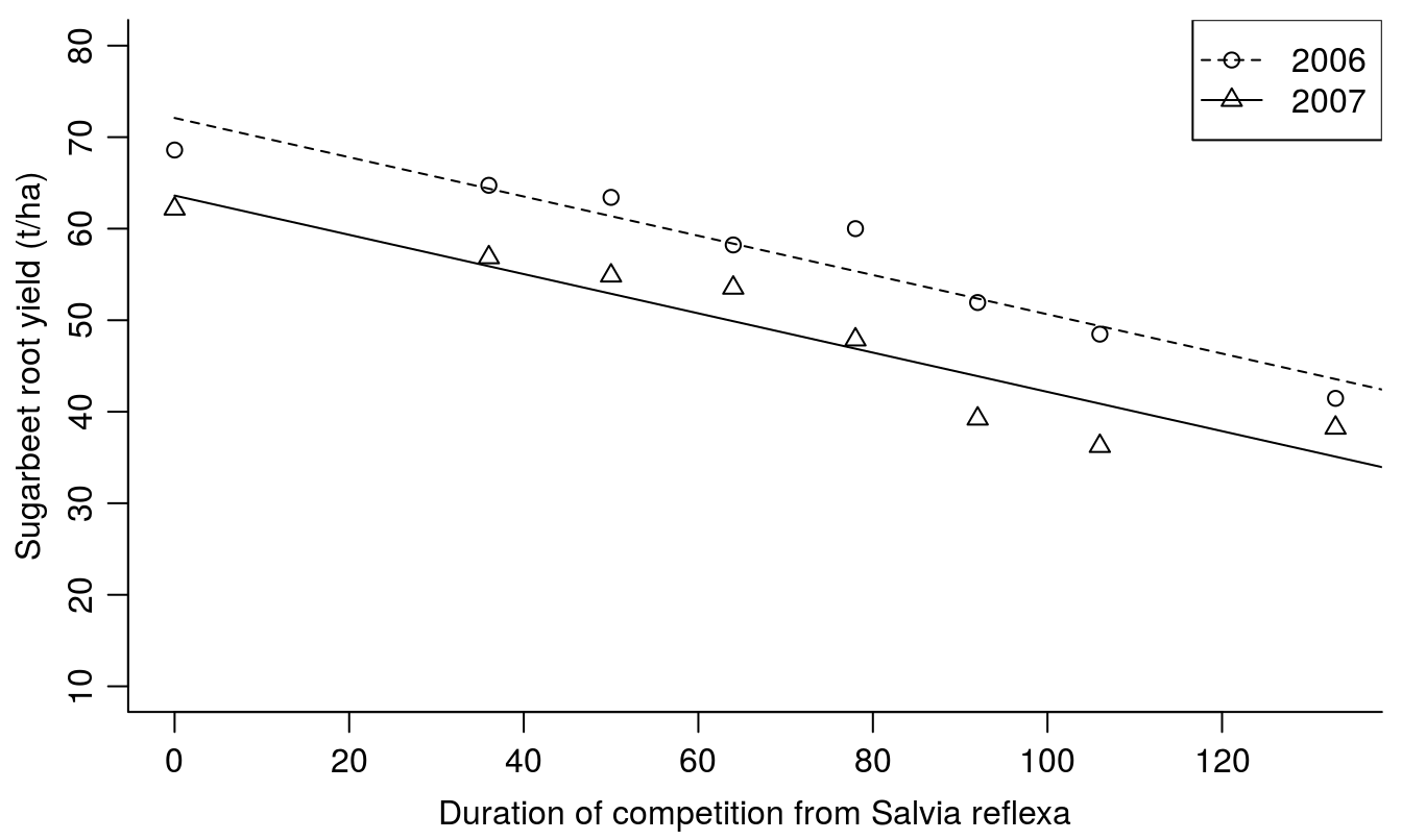
Figure 7.5: Sugarbeet yield in response to duration of Salvia reflexa competition.
Note the codes to obtain the regression lines for each year are more involved that in the harrowing example in Figure 7.3. You must separate the regression lines on the basis of Year and define an independent variable x. Since it is a strait line you only need two `x’s within year to draw the lines.
Even though the maximum yield (y-intercept) was different between years (72.1 in 2006 compared with 63.6 in 2007), yield reduction was similar in response to duration of weed competition. Each day of competition reduced the yield by 0.21 tons/ha (slope= -0.215 (0.025)).