6 Linear Regression
6.1 Simple Linear Regression
Linear regression in R is very similar to analysis of variance. In fact, the mathematics behind simple linear regression and a one-way analysis of variance are basically the same. The main difference is that we use ANOVA when our treatments are unstructured (say, comparing 5 different pesticides or fertilizers), and we use regression when we want to evaluate structured treatments (say, evaluating 5 different rates of the same pesticide or fertilizer). In linear regression, we will use the lm() function instead of the aov() function that was used in the ANOVA chapter. However, it should be noted that the lm() function can also be used to conduct ANOVA. The primary advantage of aov() for ANOVA is the ability to incorporate multi-strata error terms (like for split-plot designs) easily.
To illustrate linear regression in R, we will use data from (Kniss et al. 2012), quantifying the sugar yield of sugarbeet in response to volunteer corn density. The response variable is sucrose production in pounds/acre (LbsSucA), and the independent variable is volunteer corn density in plants per foot of row. The lm() function syntax (for the purpose of regression) requires a formula relating the response variable (Y) to independent variable(s), separated by a ~, for example: lm(Y ~ X).
beets.dat <- read.csv("http://rstats4ag.org/data/beetvolcorndensity.csv")
head(beets.dat)
## Loc Density LbsSucA
## 1 WY09 0.00 10106.34
## 2 WY09 0.03 8639.42
## 3 WY09 0.05 7752.20
## 4 WY09 0.08 5718.38
## 5 WY09 0.11 7953.72
## 6 WY09 0.15 6012.16density.lm <- lm(LbsSucA ~ Density, data = beets.dat)6.1.1 Model Diagnostics
The assumptions can be checked in the same manner as with the fitted aov object (see ANOVA section for full details). Quick diagnostic plots can be obtained by plotting the fitted lm object.
par(mfrow=c(1,2), mgp=c(2,.7,0), mar=c(3.2,3.2,2,.5))
plot(density.lm, which=1:2)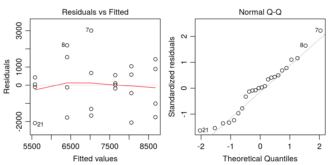
Figure 6.1: Model diagnostic plots for linear model of sugarbeet yield as a function of volunteer corn density.
We can also conduct a lack-of-fit test to be sure a linear model is appropriate. The simplest way to do this is to fit a linear model that removes the linear structure of the independent variable (treating it as a factor variable). The models can then be compared using the anova() function.
density.lm2 <- lm(LbsSucA ~ as.factor(Density), data = beets.dat)
anova(density.lm, density.lm2)
## Analysis of Variance Table
##
## Model 1: LbsSucA ~ Density
## Model 2: LbsSucA ~ as.factor(Density)
## Res.Df RSS Df Sum of Sq F Pr(>F)
## 1 22 42066424
## 2 18 40058981 4 2007444 0.2255 0.9206When 2 linear models are provided to the anova() function, the models will be compared using an F-test. This is only appropriate when the models are nested; that is, one model is a reduced form of the other. The highly non-significant p-value above (p = 0.92) indicates that removing the structured nature of the density variable does not increase the model fit. Therefore, we will proceed with the regression analysis.
6.1.2 Model Interpretation
Using the anova() function on a a single fitted lm object produces output similar to the aov() function. The ANOVA table indicates strong evidence that volunteer corn density has an effect on the sugar production, as expected. To get the regression equation, we use the summary() function on the fitted lm model:
anova(density.lm)## Analysis of Variance Table
##
## Response: LbsSucA
## Df Sum Sq Mean Sq F value Pr(>F)
## Density 1 25572276 25572276 13.374 0.001387 **
## Residuals 22 42066424 1912110
## ---
## Signif. codes: 0 '***' 0.001 '**' 0.01 '*' 0.05 '.' 0.1 ' ' 1summary(density.lm)##
## Call:
## lm(formula = LbsSucA ~ Density, data = beets.dat)
##
## Residuals:
## Min 1Q Median 3Q Max
## -2086.02 -1084.01 23.92 726.23 3007.73
##
## Coefficients:
## Estimate Std. Error t value Pr(>|t|)
## (Intercept) 8677.6 485.6 17.869 1.38e-14 ***
## Density -20644.7 5645.2 -3.657 0.00139 **
## ---
## Signif. codes: 0 '***' 0.001 '**' 0.01 '*' 0.05 '.' 0.1 ' ' 1
##
## Residual standard error: 1383 on 22 degrees of freedom
## Multiple R-squared: 0.3781, Adjusted R-squared: 0.3498
## F-statistic: 13.37 on 1 and 22 DF, p-value: 0.001387The resulting output provides estimates for the intercept (8678), and slope (-20645) of the regression line under the heading “Coefficients.” The summary() function also prints standard errors, t-statistics, and P-values, and fit statistics such as the R2 for these estimates are also provided. The regression line for this example would be:
Y = 8678 - 20645*X
To plot the data along with the fitted line:
par(mfrow=c(1,1), mar=c(3.2,3.2,2,.5), mgp=c(2,.7,0))
plot(beets.dat$LbsSucA ~ beets.dat$Density, bty="l",
     ylab="Sugar yield (lbs/A)", xlab="Volunteer corn density (plants/ft row)",
     main="Lingle, WY 2009", ylim=c(0,10000))
  abline(density.lm) # Add the regression line
# to add the regression equation into the plot:
  int<-round(summary(density.lm)$coefficients[[1]]) # get intercept
  sl<- round(summary(density.lm)$coefficients[[2]]) # get slope
  reg.eq<-paste("Y =", int, sl, "* X") # create text regression equation
  legend("bottomleft",reg.eq, bty="n")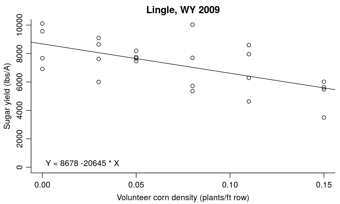
Figure 6.2: Effect of volunteer corn density on sugarbeet yield.
The sugar yield was decreased by 20,600 lbs/A for each volunteer corn plant per foot of sugarbeet row; this seems unintuitive since the Y-intercept was only 8,678 lbs/A. The maximum volunteer corn density used in the study was only 0.15 plants per foot of sugarbeet row, so the units of the slope are not directly applicable to the data observed in the study. Although the linear regression model is appropriate here, it is extremely important not to extrapolate the linear model results to volunteer corn densities outside the observed data range (densities greater than 0.15 plants per foot of row). This can be illustrated by changing the Y and X limits on the figure. If extrapolation is absolutely necessary, a nonlinear model would be more appropriate (although still not ideal). The ideal situation would be to repeat the study with weed densities that caused crop yield to drop close to the minimum yield.
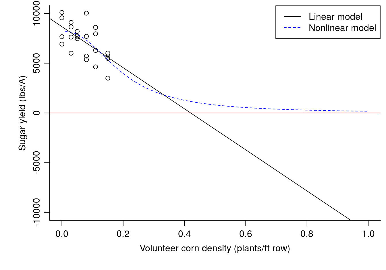
Figure 6.3: Linear model vs nonlinear model for sugarbeet response to volunteer corn density.