8 Mixed Models - ANOVA
There are many examples in agronomy and weed science where mixed effects models are appropriate. In ANOVA, everything except the intentional (fixed) treatment(s), reflect random variation. This includes soil variability, experimental locations, benches in the greenhouse, weather patterns between years; many things can affect experimental results that simply cannot be controlled. In many cases, we can try to account for these sources of variation by blocking. We can consider the selection of the blocks to take place at random in the sense that we usually cannot tell in advance whether or not the next block will exhibit a low, high, or more moderate response level. In this context, we can describe random effects as effects that cannot be controlled and therefore cannot be explained by the treatment structure of the experiment. In many designed experiments, we are not inherently interested in these random effects, but in an adequate analysis we need to acknowledge the variation that they contribute. We can do so using a mixed effects model that contains both fixed and random effects.
To illustrate mixed effects ANOVA, we will use the same dry bean herbicide data set that was used in the ANOVA section to allow for comparison; please read the ANOVA section for details on the study. We will need to load the lme4 and multcomp packages for this analysis.
library(lme4)
read.csv("http://rstats4ag.org/data/FlumiBeans.csv")->flum.dat
flum.dat$yrblock  <- with(flum.dat, factor(year):factor(block))
First, we can look at group means (in plants per acre, and plants per hectare) using the dplyr package.
library(dplyr)
beansum <- flum.dat %>%
  group_by(year, treatment) %>%
  summarize( Pop.plantsA  = round(mean(population.4wk),-2),
             Pop.plantsHa = round(mean(population.4wk*2.47),-2))
beansum
## # A tibble: 21 x 4
## # Groups: year [3]
## year treatment Pop.plantsA Pop.plantsHa
## <int> <fct> <dbl> <dbl>
## 1 2009 EPTC + ethafluralin 48800 120500
## 2 2009 flumioxazin + ethafluralin 38300 94700
## 3 2009 flumioxazin + pendimethalin 19700 48800
## 4 2009 flumioxazin + trifluralin 24400 60300
## 5 2009 Handweeded 34800 86100
## 6 2009 imazamox + bentazon 49900 123400
## 7 2009 Nontreated 46500 114800
## 8 2010 EPTC + ethafluralin 56600 139900
## 9 2010 flumioxazin + ethafluralin 15700 38700
## 10 2010 flumioxazin + pendimethalin 20000 49500
## # … with 11 more rows8.1 Mixed Effects Model using the lme4 Package
In the ANOVA section, we considered year, block, and treatment all as fixed effects. However, because the number of replicates was different by year, analyzing the combined data from all three years is problematic. The effect of year is unbalanced; we have more observations for 2010 and 2011 than for 2009. We can deal with the unbalanced nature of the data by using a mixed effects model. There are other good reasons for analyzing the data as a mixed effect model. The hope is that the results of this experiment can be generalized beyond the three years the study was conducted. The three years in which we conducted the experiment represent 3 possible years out of many when the experiment could have been done, and therefore, we can assume the impact of year to be a random variable. Same goes for the blocking criteria within a year. However, the treatments were selected specifically to determine their impact on the dry bean crop. Therefore, we will consider the treatments as fixed effects, but the year and blocking criteria within a year random effects.
# Mixed Effects ANOVA
lmer(population.4wk ~ treatment+(1|year/block), data=flum.dat, REML=F)->flum.lmer
## boundary (singular) fit: see ?isSingularanova(flum.lmer)## Analysis of Variance Table
## Df Sum Sq Mean Sq F value
## treatment 6 1.1974e+10 1995718507 28.8878.1.1 Model Comparison and Obtaining P-values
One of the most frustrating things to many researchers analyzing mixed models in R is a lack of p-values provided by default. The calculation of P-values for complex models with random effects and multiple experimental unit sizes is not a trivial matter. Certain assumptions must be made, and it is difficult to generalize these assumptions from experiment to experiment. Therefore, the authors of the lme4 package have chosen not to print P-values by default. We can get a P-value for the fixed effect of treatment in two different ways. First, we can compare our model with a reduced model that does not contain the treatment effect. The P-value that results, then, is effectively the P-value for the treatment effect. When comparing lmer() models, it is important to specify the argument REML=F in both models so that the model is fit using full maximum likelihood (rather than the default restricted maximum likelihood).
lmer(population.4wk ~ (1|year/block), data=flum.dat, REML=F)->flum.null # reduced model
anova(flum.null, flum.lmer) # anova function to compare the full and reduced models
## Data: flum.dat
## Models:
## flum.null: population.4wk ~ (1 | year/block)
## flum.lmer: population.4wk ~ treatment + (1 | year/block)
## Df AIC BIC logLik deviance Chisq Chi Df Pr(>Chisq)
## flum.null 4 1710.4 1719.8 -851.20 1702.4
## flum.lmer 10 1633.0 1656.5 -806.52 1613.0 89.359 6 < 2.2e-16 ***
## ---
## Signif. codes: 0 '***' 0.001 '**' 0.01 '*' 0.05 '.' 0.1 ' ' 1A second method for getting a p-value for fixed effects is to use the Anova() (note the different capitalization) from the car package. This will provide an anova table of the full model that is complete with p-values. By deault, the Anova() function will provide p-values from a Chi-square test.
# Mixed Effects ANOVA - with p-values from Chisq test:
library(car)
Anova(flum.lmer) # Chi-square
## Analysis of Deviance Table (Type II Wald chisquare tests)
##
## Response: population.4wk
## Chisq Df Pr(>Chisq)
## treatment 173.32 6 < 2.2e-16 ***
## ---
## Signif. codes: 0 '***' 0.001 '**' 0.01 '*' 0.05 '.' 0.1 ' ' 1To get a p-value from an F-test, the model must be fit using restricted maximum likelihood.
# re-fit the model with REML, and get F-test:
lmer(population.4wk ~ treatment+(1|year/block),
     data=flum.dat, REML=T)->flumREML.lmer #note REML = TRUE
Anova(flumREML.lmer, test="F") # F-test
## Analysis of Deviance Table (Type II Wald F tests with Kenward-Roger df)
##
## Response: population.4wk
## F Df Df.res Pr(>F)
## treatment 26.537 6 60 3.518e-15 ***
## ---
## Signif. codes: 0 '***' 0.001 '**' 0.01 '*' 0.05 '.' 0.1 ' ' 1For this example, treatment effect produces a very low p-valueregardless of method we use to get it, indicating there appears to be a strong effect of treatment on dry bean emergence Therefore, we will want to look at the treatment means to determine which treatments affected dry bean stand. First, though, it is often of interest to look at the random effects.
8.1.2 Random Effects
The summary() function can be used to print most of the relevant information from the mixed model fit summary(flum.lmer). We can selectively print only the certain parts of the model fit. Adding $varcor to the summary function of the fit will print out the variance components for the random terms as well as the residual variance.
summary(flum.lmer)$varcor## Groups Name Std.Dev.
## block:year (Intercept) 0.0
## year (Intercept) 3145.8
## Residual 8311.9The random ‘year’ effect appears to be contributing substantially to the model, but the blocking criteria within a year does not. When reporting results of a random effects model for publication, it is important that these results be included so that a full accounting of variability is provided. The ranef() function returns estimates for the random effects of year:
ranef(flum.lmer)$year## (Intercept)
## 2009 1364.250
## 2010 2517.688
## 2011 -3881.937On average, bean populations were lowest in 2011, and highest in 2010. Using tapply() results in a similar conclusion, and helps put the random effects estimates into context.
tapply(flum.dat$population.4wk, flum.dat$year, mean) ## 2009 2010 2011
## 37503.00 38830.64 30835.398.1.3 Fixed Effects & Mean Separation
In most designed agricultural experiments, the fixed effects (and specifically differences between fixed effects treatments) are of most interest to the researcher. We can use the glht() function in the multcomp package to separate treatment means if we conclude there is a significant treatment effect. The p-values below are adjusted using Tukey’s method.
library(multcomp)
summary(glht(flum.lmer, linfct=mcp(treatment="Tukey")))->flum.glht
flum.glht # print all pairwise comparisons
Printing all pairwise comparisons is valuable to get P-values, estimates of differences, etc. for reporting (not shown here due to space). But we can also plot the 95% confidence intervals to allow better visualization of differences. In Figure 8.1, the comparison is listed on the left in the format (treatment1 - treatment2). If the confidence interval bars do not include zero (the vertical dotted line) then one could conclude that difference between treatments is significantly different according to the Tukey adjusted p-values (at the 5% confidence level).
par(mar=c(5,22,3,1), mgp=c(2,.7,0)) # set wide left margin
plot(flum.glht)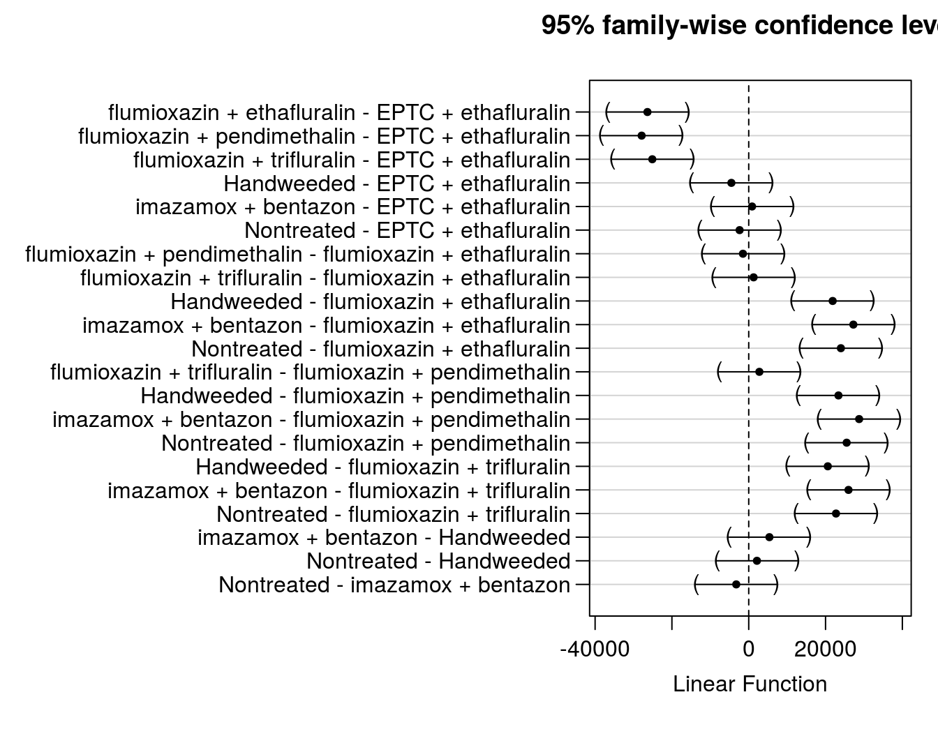
Figure 8.1: Model estimates of treatment differences with 95% confidence intervals.
The glht() function will not allow for unadjusted comparisons, since multiple testing tends to inflate the likelihood of a Type I error. If for some reason unadjusted Fisher LSD p-values are required (similar to the default in SAS) the emmeans() function in the emmeans package can be used. The estimated mrginal means (or least-square means) cna be printed along with the mean separation groups using the cld() function from the multcomp package, and the pairwise comparisons of estimated marginal means can be printed by calling the ‘contrasts’ of the estimated marginal means.
library(emmeans)
emmeans(flum.lmer, pairwise ~ treatment, data=flum.dat, adjust="none") -> flum.emm
multcomp::cld(flum.emm$emmeans)
## treatment emmean SE df lower.CL upper.CL .group
## flumioxazin + pendimethalin 20003 3483 20.9 12757 27250 1
## flumioxazin + ethafluralin 21508 3483 20.9 14262 28754 1
## flumioxazin + trifluralin 22775 3483 20.9 15529 30022 1
## Handweeded 43368 3483 20.9 36122 50614 2
## Nontreated 45506 3483 20.9 38260 52752 2
## EPTC + ethafluralin 47882 3483 20.9 40636 55128 2
## imazamox + bentazon 48753 3483 20.9 41507 55999 2
##
## Degrees-of-freedom method: kenward-roger
## Confidence level used: 0.95
## P value adjustment: tukey method for comparing a family of 7 estimates
## significance level used: alpha = 0.05flum.emm$contrasts## contrast estimate SE df t.ratio p.value
## EPTC + ethafluralin - flumioxazin + ethafluralin 26374 3698 71.1 7.132 <.0001
## EPTC + ethafluralin - flumioxazin + pendimethalin 27879 3698 71.1 7.539 <.0001
## EPTC + ethafluralin - flumioxazin + trifluralin 25107 3698 71.1 6.790 <.0001
## EPTC + ethafluralin - Handweeded 4514 3698 71.1 1.221 0.2262
## EPTC + ethafluralin - imazamox + bentazon -871 3698 71.1 -0.236 0.8144
## EPTC + ethafluralin - Nontreated 2376 3698 71.1 0.643 0.5226
## flumioxazin + ethafluralin - flumioxazin + pendimethalin 1505 3698 71.1 0.407 0.6853
## flumioxazin + ethafluralin - flumioxazin + trifluralin -1267 3698 71.1 -0.343 0.7328
## flumioxazin + ethafluralin - Handweeded -21859 3698 71.1 -5.911 <.0001
## flumioxazin + ethafluralin - imazamox + bentazon -27245 3698 71.1 -7.368 <.0001
## flumioxazin + ethafluralin - Nontreated -23998 3698 71.1 -6.490 <.0001
## flumioxazin + pendimethalin - flumioxazin + trifluralin -2772 3698 71.1 -0.750 0.4559
## flumioxazin + pendimethalin - Handweeded -23364 3698 71.1 -6.318 <.0001
## flumioxazin + pendimethalin - imazamox + bentazon -28750 3698 71.1 -7.775 <.0001
## flumioxazin + pendimethalin - Nontreated -25503 3698 71.1 -6.897 <.0001
## flumioxazin + trifluralin - Handweeded -20592 3698 71.1 -5.569 <.0001
## flumioxazin + trifluralin - imazamox + bentazon -25978 3698 71.1 -7.025 <.0001
## flumioxazin + trifluralin - Nontreated -22731 3698 71.1 -6.147 <.0001
## Handweeded - imazamox + bentazon -5386 3698 71.1 -1.456 0.1497
## Handweeded - Nontreated -2138 3698 71.1 -0.578 0.5649
## imazamox + bentazon - Nontreated 3247 3698 71.1 0.878 0.3828
##
## Degrees-of-freedom method: kenward-roger