3 Simple Correlation

To quantify relationships between quantitative treatment structures (such as increasing rates) and a response variable, regression analysis is most appropriate. But in many cases it is of interest to determine the strength of a relationship between two measured variables (where no cause-effect or dose-response relationship is obvious). This can most easily be done with correlation analysis. Examples where correlation analysis would be appropriate include observational studies where soil texture (e.g. percent clay content) is thought to be related to density of a particular weed species; or the amount of sunlight reaching the crop canopy is related to crop biomass. In these cases, experimental treatments may not be explicitly designed, but rather many areas of a field could be sampled for both variables, and the correlation analysis conducted to quantify the strength of the relationship. The relationship between visual assessment of crop injury and dry weight (or yield) production of a crop may also be of interest to a researcher. This would not be a cause-effect relationship (injury symptoms do not cause dry weight reduction), and therefore correlation analysis is more appropriate than regression. In a study by Lyon and Kniss (2010), proso millet was tested for its tolerance to preemergence applications of the herbicide saflufenacil. Injury to the crop was evaluated visually at 10 and 20 days after treatment, and dry weight was measured 28 days after treatment. It is expected that visual injury symptoms would have a strong (negative) relationship with dry weight production; however, exceptions to this relationship may exist. Correlation analysis can be conducted in R using the cor.test function.

read.csv("http://rstats4ag.org/data/millet.csv")->millet.dat
cor.test(millet.dat$injury.10dat,millet.dat$drywt)

## 
##  Pearson's product-moment correlation
## 
## data:  millet.dat$injury.10dat and millet.dat$drywt
## t = -12.529, df = 407, p-value < 2.2e-16
## alternative hypothesis: true correlation is not equal to 0
## 95 percent confidence interval:
##  -0.5941612 -0.4538439
## sample estimates:
##        cor 
## -0.5275917

cor.test(millet.dat$injury.20dat,millet.dat$drywt)

## 
##  Pearson's product-moment correlation
## 
## data:  millet.dat$injury.20dat and millet.dat$drywt
## t = -14.724, df = 411, p-value < 2.2e-16
## alternative hypothesis: true correlation is not equal to 0
## 95 percent confidence interval:
##  -0.6474176 -0.5206627
## sample estimates:
##        cor 
## -0.5876339

Both injury evaluations were highly correlated (P<0.0001) to dry weight. The 20 day evaluation had a stronger relationship with dry weight (r=-0.59) compared with the 10 day evaluation (r=-0.53). This would be expected as the 20 day evaluation was taken only 8 days before the plants were harvested for dry weight.

The output from cor.test also indicates that Pearson’s correlation was used, which is the default correlation method, and in this case is appropriate. The cor.test function can also conduct Kendall and Spearman correlation, simply by adding the “method” as an argument within the function:

var1<-1:5
var2<-2:6
cor.test(var1, var2, method="kendall") 

## 
##  Kendall's rank correlation tau
## 
## data:  var1 and var2
## T = 10, p-value = 0.01667
## alternative hypothesis: true tau is not equal to 0
## sample estimates:
## tau 
##   1

cor.test(var1, var2, method="spearman")

## 
##  Spearman's rank correlation rho
## 
## data:  var1 and var2
## S = 4.4409e-15, p-value = 0.01667
## alternative hypothesis: true rho is not equal to 0
## sample estimates:
## rho 
##   1

The pairs function allows a quick method for visualizing relationships between variables. In the example below, the 4th through 6th data columns (both injury evaluations and dry weight) are included in pairwise scatterplots.

par(cex=2, mgp=c(2,.7,0))
pairs(millet.dat[4:6], pch=19, col=rgb(red=0.1, green=0.1, blue=0.1, alpha=0.2))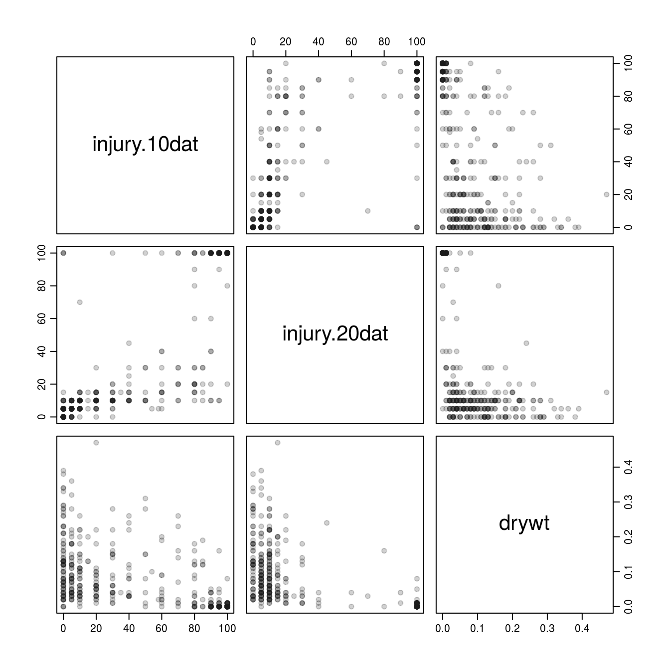

Figure 3.1: Relationship between injury and dry weight using the pairs() function.

---