12 Nonlinear Regression - Selectivity of Herbicides

Herbicides are unique in that they are designed to kill plants. Sufficiently high doses will kill both crops and weeds, while small doses have no effect on crops and weeds. For the selective herbicides there are dose-range windows that control some weeds without harming the crop too much. The action of a herbicide is usually determined by its chemical and physical properties, its effect on plant metabolism, the stage of development of the plant and the environment. The purpose of this chapter is to give an overview of the basic principles of how to quantitatively assess herbicide selectivity.

The chapter is based upon general toxicology commonly used in many disciplines of the biological sciences and it is also used to classify xenobiotics according to their toxic profile; the first of which is the dose required to kill 50% of some test animals (e.g., rats, mice, hamsters). However, the principles in the pesticide science have focus not only on general toxicity, but also on selectivity, particularly when it comes to herbicides.

12.1 Dose-Response Curves

The difference between tolerance and control of a plant is determined by the size of the dose. The term size of a dose, however, is rather vague in that for some herbicides, only few g/ha are needed to control weeds (e.g., many sulfonylureas) whereas for others we must apply several kg to obtain the same level of control (e.g., phenoxy acids). If we want to determine the potency or selectivity of a herbicide it is not enough only to look at one dose-response curve, as the proper assessment of selectivity should be stated in relative terms depending on the herbicide, crops and weeds in question. In order to avoid ambiguity in assessment of selectivity the sigmoid log-logistic dose-response curve is a good starting point.

\[y=c+\frac{d-c}{1+ \left(\frac{x}{ED_{50}}\right)^b} \]

Where y is the response, d denotes the upper limit, c the lower limit, $ED_{50}$ denotes the dose, x, required to half the response 50% between d and c. Finally b denotes the relative slope of the curve around $ED_{50}$.

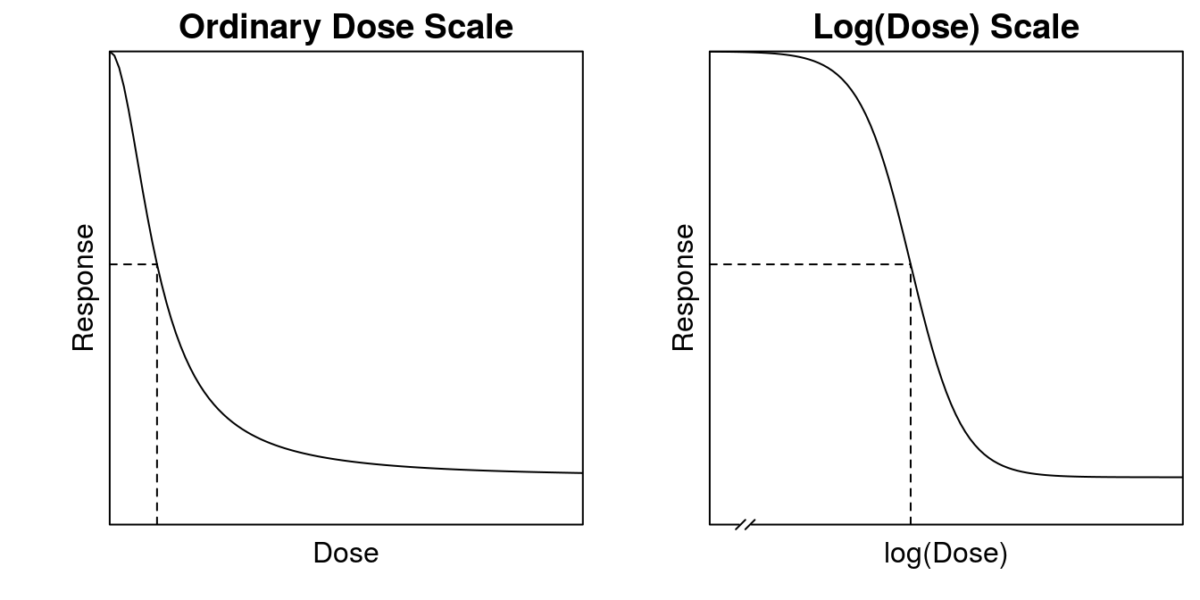
$The log-logistic curve plotted on ordinary dose axis and log(Dose) axis. The broken lines indicate the $ED_{50}$ on the x-axis and on the y-axis. The broken line on the log(Dose axis) indicates that a zero-dose does not exist on a logarithmic axis.$

Figure 12.1: The log-logistic curve plotted on ordinary dose axis and log(Dose) axis. The broken lines indicate the $ED_{50}$ on the x-axis and on the y-axis. The broken line on the log(Dose axis) indicates that a zero-dose does not exist on a logarithmic axis.

The ordinary dose-scale looks almost as an exponential decay curve apart form the upper part where there is a small bend. However, one of the nice properties of the log-logistic curves is that it is symmetric on the log(dose) scale (Figure 12.1). The inflection point is the $ED_{50}$ whatever the dose scale. The broken lines in Figure 12.1 show the location of $ED_{50}$, and in equation 1 it is a natural parameter of the model. If zero-dose is used as control we must break the x-axis to indicate that the logarithm to zero does not exist.

12.2 Assessment of Selectivity

If we want to compare the phytotoxicity of two or more herbicides on the same plant species or maybe the selectivity of a herbicide upon a crop and a weed species, then we must compare several dose-response curves simultaneously and quantify our findings in relative terms. We must define a standard herbicide and/or a standard species.

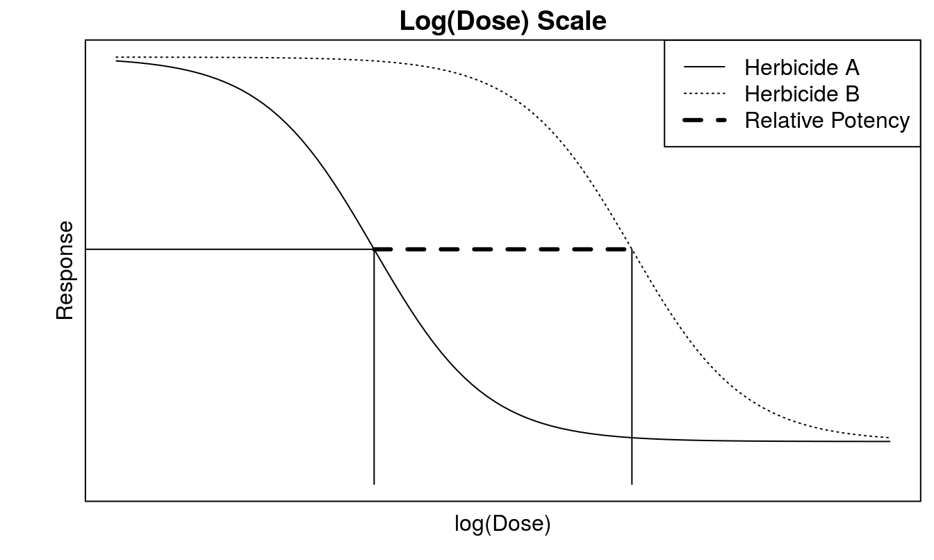
$The relative potency at $ED_{50}$ is the distance between the two curves. Note that the doses are on log scale and therefore the distance shown at the graph is the ratio between the two doses. In this instance the two curves are similar, i.e. that they have the same upper and lower limit and slope. It is only the $ED_{50}$ that differs.$

Figure 12.2: The relative potency at $ED_{50}$ is the distance between the two curves. Note that the doses are on log scale and therefore the distance shown at the graph is the ratio between the two doses. In this instance the two curves are similar, i.e. that they have the same upper and lower limit and slope. It is only the $ED_{50}$ that differs.

To make things simple we assume that we compare the action of two herbicides on the same plant species or at different plant species but with the same upper limit, d, and lower limit c.

The distance between the two dose-response curves at $ED_{50}$ is a measure of the biological exchange rate between herbicides (Figure 12.2), analogous to the more common practice of exchanging currencies, when traveling to foreign land. In toxicology and herbicide selectivity, we do not call it exchange rate, but the relative potency or relative strength, and when studying herbicide resistant biotypes of weeds, the resistance factor or R:S ratio.

For example, we know that to get adequate control of a common weed flora we need $x_{B}$ g of a test herbicide and $x_{A}$ g of the standard herbicide per unit area. Some will argue that $ED_{50}$ is not at all of interest when it comes to controlling weeds, since we are never interested in only achieving 50% control. While true from a practical standpoint, for the time being we will look at $ED_{50}$ because it is a natural parameter of the log-logistic curve, and therefore it is an important parameter to classify toxic material. Later, we will look at the two additional ED-levels - $ED_{10}$ to assess the crop tolerance and $ED_{90}$ to assess the weed control. In general terms, we can define the relative potency as a response half way between the upper limit,d, and the lower limit c.

\[ R=\frac{x_{A}}{x_{B}} \]

Where the relative potency, R, can be defined at any $ED_{x}$ level of which $ED_{10}$, $ED_{50}$, and $ED_{90}$ are the most common levels in Weed Science. In ecotoxicology $ED_{05}$ is common to define an no-effect level.

If the relative potency, R=1.0, then there is no difference between the effect of the two herbicides, i.e. $x_{A}$ = $x_{B}$, if R<1 the herbicide dose of B is less effective than herbicide A and if R>1 the herbicide A is more effective than herbicide B. So every time we calculate the relative potency, then we must know if the sheer ratio is different from 1.0.

In Figure 12.2, the two dose response curves are similar in that the upper and lower limit are the same for the two curves as are the relative slopes, b. But what if the two curves are not similar (and this more commonly the rule rather than the exception in real life)?

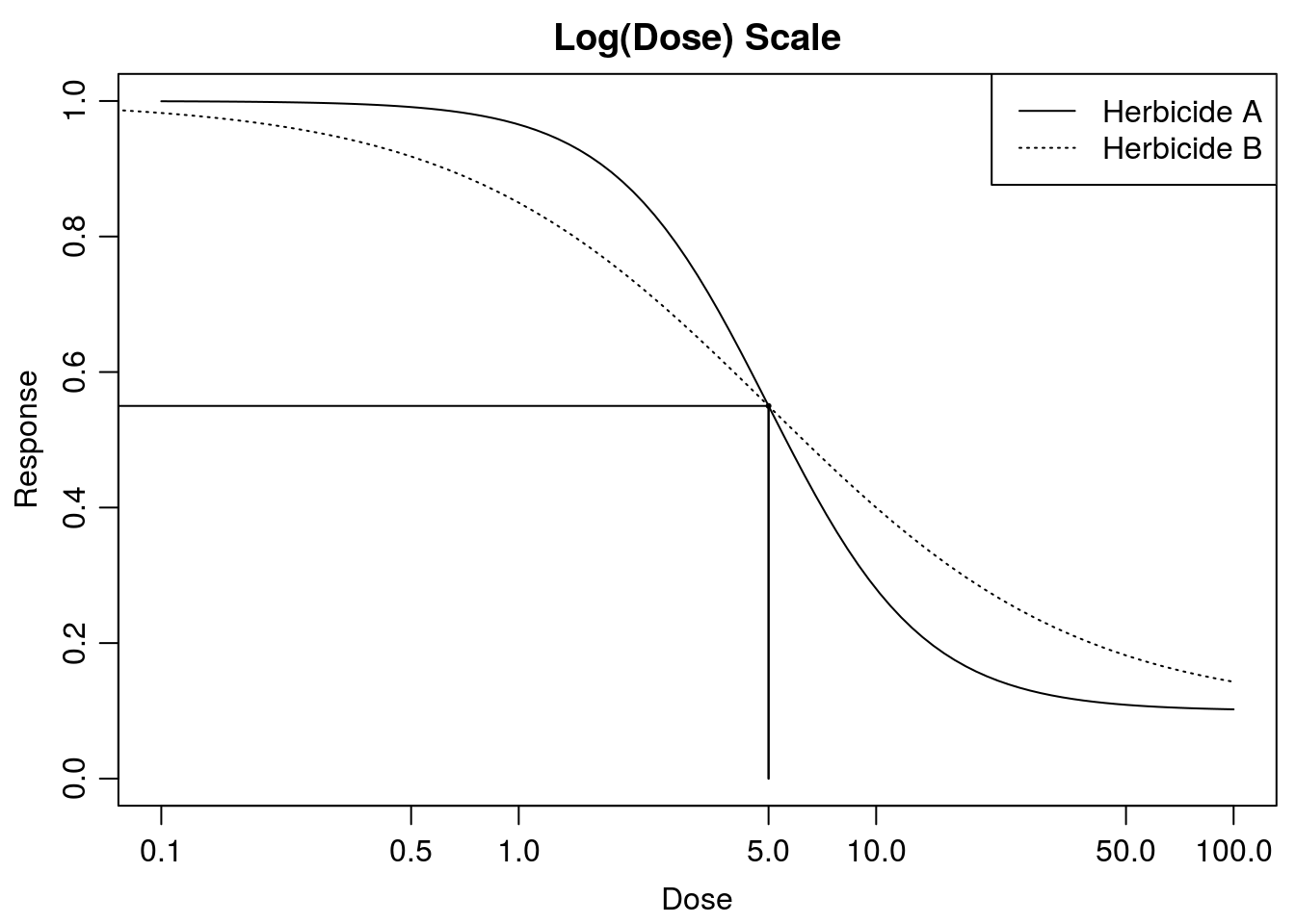
$The two herbicides have similar upper and lower limit and $ED_{50}$, but have different slopes.$

Figure 12.3: The two herbicides have similar upper and lower limit and $ED_{50}$, but have different slopes.

It is evident that in some cases $ED_{50}$ does not give the right picture of toxicity when curves are not similar (Figure 12.3). Herbicide A is less potent above $ED_{50}$ and more potent below $ED_{50}$. Consider the example in Figure 12.3 where the slopes are different but the $ED_{50}$ s are identical. How should we report this? One way of doing it is to report the relative potency at relevant response levels. By defining Herbicide A as being the standard, it means that its $ED_{x}$ is in the denominator. We get the following relative potencies:

## 
## Estimated effective doses
## 
##          Estimate Std. Error
## e:1:10 1.6667e+00 3.6316e-07
## e:1:50 5.0000e+00 5.1752e-07
## e:1:90 1.5000e+01 3.5880e-06

## 
## Estimated effective doses
## 
##          Estimate Std. Error
## e:1:10 5.5556e-01 1.7824e-07
## e:1:50 5.0000e+00 1.2011e-06
## e:1:90 4.5000e+01 2.6206e-05

##    e:1:10    e:1:50    e:1:90 
## 2.9999968 1.0000014 0.3333346

Herbicide A the doses are 1.67, 5, 15` for $ED_{10}$, $ED_{50}$ and $ED_{90}$, respectively.
Herbicide B the doses are 0.56, 5, 45 for $ED_{10}$, $ED_{50}$ and $ED_{90}$,respectively.
And the relative potencies are 3, 1, 0.33 at $ED_{10}$, $ED_{50}$ and $ED_{90}$, respectively when Herbicide A is the standard.

Note how the relative potency changes from 3.0 at $ED_{10}$ to 0.33 at $ED_{90}$. Above $ED_{50}$ herbicide B is more potent than herbicide A, but this changes below $ED_{50}$ where the herbicide A now is most potent. This problem is looked at in more detailed in the previous chapter on dose response curves.

The $ED_{50}$ somewhat resembles the $LD_{50}$ (or dose required to cause 50% mortality in a test population) as an estimate in acute toxicity in toxicology, it does not tell the full story in Weed science. Particularly, when we wish to compare the selectivity of a herbicide on a crop and a weed flora, be it predominant weed species or not. $ED_{50}$ contains much more information than do $LD_{50}$, but becomes more difficult to interpret because we typically deal with continuous responses in Weed Science.

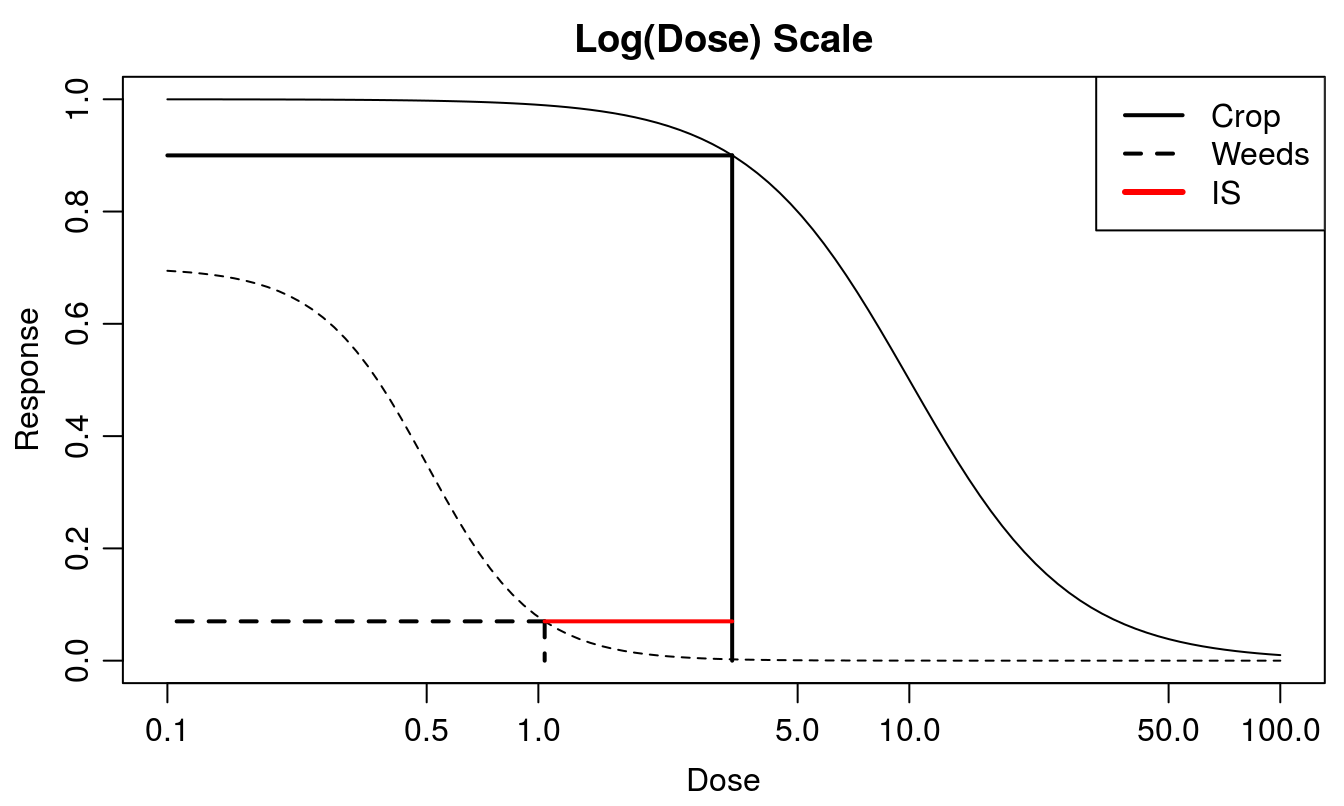
Figure 12.4: The assessment of the Selectivity Index for a crop and a weed or a group of weeds.

12.3 Selectivity index

Since herbicides may have an effect on any plant, be it crop or weeds, we sometimes have to accept a small decrease in the yield of the crop growing in a weed free environment. For example a 10% decrease might be tolerated, $ED_{10}$, while a 90% control of the weed, $ED_{90}$, is considered a reasonable control level of the weeds. The $ED_{10}$ for the crop is 3.33 and the $ED_{90}$ for the weed is 1.04. Consequently the Selectivity Index is 3.20. As seen in Figure 12.4, the upper limits for the crop and the weed are different.

In the development of herbicides the companies screen virtually 10,000’s of compounds, only a small fraction of which may have some activity. In order to handle this immense amount of information, they must unambiguously define the selectivity of herbicides in the development phase. By accepting a 10% yield loss of the crop growing in weed free environment and by being satisfied with a 90% effect on the weeds growing in crop free environment, we get an Index of Selectivity, IS:

\[ IS=\frac{{[ED_{10}]_{crop}}}{{[ED_{90}]_{weeds}}} \]

However, the same situation arises when we compare herbicide resistant biotypes with susceptible biotypes. Obviously, if there is target site resistance and a yield penalty we expect difference in response in untreated control. If it is metabolic resistance where no yield penalty has been observed, we can still have different untreated control response. This fact of differences in upper limit among curves are not being solved by making the untreated control equal to 100 and adjust the responses within biotypes accordingly. This often-ignored problem is dealt with in the previous chapter on dose-response curves.

12.4 Vertical and Horizontal Assessment

Vertical and horizontal assessment of herbicide effect is shown graphically in Figure 12.5.

12.4.1 Vertical assessment

Vertical assessment compares plant response at some preset dose levels. This is the most common method for evaluating herbicides in the field. If doses were chosen close to the upper or lower limit of the curves, differences between treatments would be less than if they were chosen in the middle part of the curve. If we are only working at dose-ranges in the middle part of the curves then, in this particular instance, differences would be almost independent of dose-levels. Consequently, the middle region is obviously the optimal part of the curve to obtain information about differences of effects in this particular graph where the curves are looking very similar. This, however, does not apply when the curves have different slopes as shown in Figure 12.4.

The curves show that if a herbicide is tested with or without an adjuvant in a factorial experiment, we may get significant interactions, because the differences of effects are not constant. As this interaction is dose dependent due to the S-shaped curves, it may be considered trivial and of little biological significance, when we appraise the selective action of the herbicide. If we choose only dose-ranges in the middle part of the curves, then differences are constant and independent of dose-levels and the interaction would disappear, i.e. the effects are additive.

12.4.2 Horizontal assessment

Horizontal assessment is the method we used in the herbicide selectivity section and it answers the question many farmers are interested in: which dose should I use of herbicide A to get the same effect as with herbicide B (the biological exchange rate of two herbicide products). Usually, herbicides are tested in two to three doses and their efficacy is compared with either the untreated control or with some standard herbicide treatment. Rarely, we have so many doses in the field that we actually are able to fit the entire dose response curve.

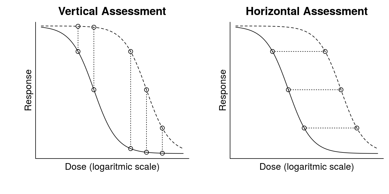
Figure 12.5: Vertical and horizontal comparison of efficacy of say two herbicide on the same plant species.

Even though the horizontal assessment above seems straight forward, it is not always the case. With continuous response variables comparing dose-response curves with different upper and lower limits is not just a trivial task to compare curves. The differences in upper and lower limits of different dose-response curves are sometimes important as they tell a story about the experiments. In the Dose-Response Curve chapter we briefly discuss it. The bottom line here is that comparison is not a matter of statistics, but a matter of biology, and thus rather complicated.