9 Mixed Models - Regression
9.1 Regression Models with Mixed Effects
When we conduct experiments over several years and/or at several locations, we have to decide if differences among years and/or differences among locations are of interest. In other words: are they fixed effects like the treatments we apply or we want to classify them random effects? If locations are picked at random it seems obvious to define locations as random effects. It means that the location contributes to the variation of the response that cannot be controlled. If the locations are picked according to their weed flora, soil type, and crop pattern, it would be wise to define locations as a fixed effect. Usually, one should use one’s common sense and the knowledge of the experimental design and the objectivewhen determining whether locations are fixed or random. There is ongoing discussions among statisticians about what should be random and what should be fixed; but that discussion is somewhat outside this course.
9.1.1 Example 1: Sugarbeet yield
Within the many years that sugarbeet has been an economic crop, we incidentally did field experiments in 2006 and 2007, near Powell, Wyoming to determine the effects of duration of Salvia reflexa (lanceleaf sage) interference with sugarbeet (Odero et al. 2010). The experiment is also used in the ANCOVA chapter.
lanceleaf.sage<-read.csv("http://rstats4ag.org/data/lanceleafsage.csv")
head(lanceleaf.sage,n=3)
## Replicate Duration Year Yield_Mg.ha Yield.loss.pct
## 1 1 36 2006 67.26 98.05
## 2 1 50 2006 60.34 87.96
## 3 1 64 2006 53.69 78.27``
First of all we look at the distribution of data within years in Figure 9.1:
library(lattice)
xyplot(Yield_Mg.ha ~ Duration | factor(Year), data = lanceleaf.sage,
    xlab="Duration of Competition",
       panel = function(x,y)
         {panel.xyplot(x,y)
          panel.lmline(x,y)})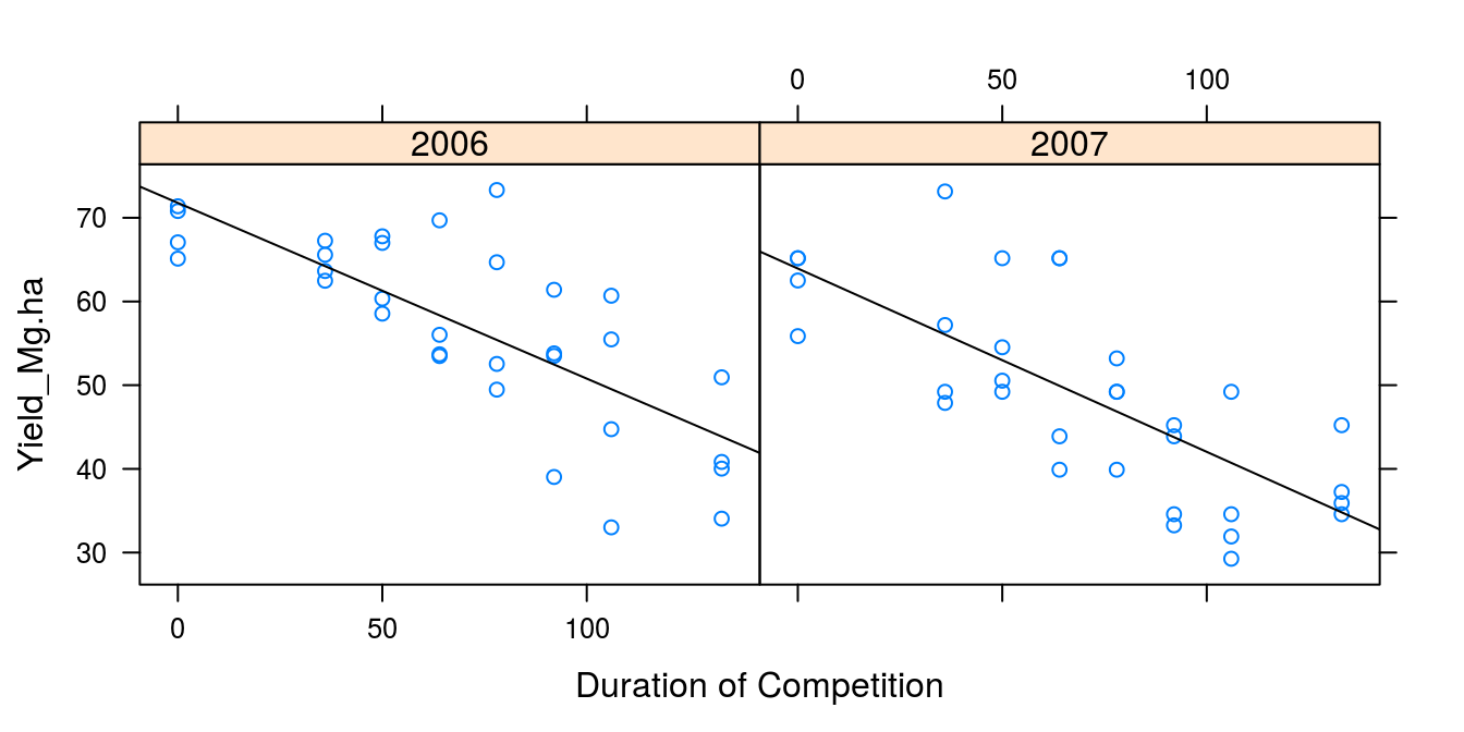
Figure 9.1: The effect of the duration of weed competition on sugarbeet yield in two different years. It looks as if the relationships could be linear.
The ANCOVA chapter analysis showed a linear regression was acceptable by checking the regression against the most general ANOVA model. The ANCOVA also showed that the regression slopes were the same independent of years, but the intercepts differed between years. In this chapter we now assume that the variation between years are random, because we cannot control the climate.
To analyze this we need to use the lmer()function in the package lme4. The syntax for lmer()is almost the same as for lm(), but there are some limitations and some important additional arguments. In lm() we can convert a continuous x-variable to a factor just by writing factor(x). You can also do that with fixed effects in the lmer()function, but when it comes to random effects you cannot. In this particular experiment, there are two random effects: experimental years (1|Year) and Replicate because it is a block experiment. But the Replicate 1 in year 2006 is not the same as Replicate 1 in 2007. Consequently, we have to make the names for Replicates unambiguously defined with a unique name, so we get a total of 8 unique levels for Year and Replicate combination and the random effect takes the form (1|New.Rep) by defining New.Rep using the with() function.
lanceleaf.sage$New.Rep <- with(lanceleaf.sage, factor(Replicate):factor(Year))
levels(lanceleaf.sage$New.Rep)
## [1] "1:2006" "1:2007" "2:2006" "2:2007" "3:2006" "3:2007" "4:2006" "4:2007"After this initial exercise, we are now ready to test whether we can assume linearity of Yield on duration of competition. We compare the regression model with the most general model, the ANOVA, as it is becoming standard practice in the course.
library(lme4)
Anova.m1 <- lmer(Yield_Mg.ha ~ factor(Duration) + (1|Year) + (1|New.Rep),
                 data=lanceleaf.sage, REML=FALSE)
Regression.m2 <- lmer(Yield_Mg.ha ~ Duration + (1|Year) + (1|New.Rep),
                      data=lanceleaf.sage, REML=FALSE)
anova(Anova.m1, Regression.m2) #No indication of nonlinearity
## Data: lanceleaf.sage
## Models:
## Regression.m2: Yield_Mg.ha ~ Duration + (1 | Year) + (1 | New.Rep)
## Anova.m1: Yield_Mg.ha ~ factor(Duration) + (1 | Year) + (1 | New.Rep)
## Df AIC BIC logLik deviance Chisq Chi Df Pr(>Chisq)
## Regression.m2 5 454.77 465.56 -222.38 444.77
## Anova.m1 11 460.97 484.72 -219.49 438.97 5.791 6 0.447The test for lack of fit is non-significant as was also seen in the ANCOVA chapter.
Notice, we have an argument that is not used in the general lm() and it is REML (Rstricted Maximum Likelihood). There are two options: Maximum Likelihood estimation (ML) REML. REML=TRUE is the default. ML produces downwards biased estimated variance components (over-optimistic precision). REML reduces the bias (similar to dividing by n - p rather than n for the residual standard error in linear regression). In other words REML agrees with lm() in case of no random effects. To make a long story short, we should use ML (REML=FALSE) when comparing models using the anova() function.
However, when we look at the summary of the mixed effect regression:
summary(Regression.m2)## Linear mixed model fit by maximum likelihood ['lmerMod']
## Formula: Yield_Mg.ha ~ Duration + (1 | Year) + (1 | New.Rep)
## Data: lanceleaf.sage
##
## AIC BIC logLik deviance df.resid
## 454.8 465.6 -222.4 444.8 59
##
## Scaled residuals:
## Min 1Q Median 3Q Max
## -1.71954 -0.65324 -0.09755 0.53285 2.36799
##
## Random effects:
## Groups Name Variance Std.Dev.
## New.Rep (Intercept) 8.994 2.999
## Year (Intercept) 14.093 3.754
## Residual 52.216 7.226
## Number of obs: 64, groups: New.Rep, 8; Year, 2
##
## Fixed effects:
## Estimate Std. Error t value
## (Intercept) 67.85642 3.40240 19.944
## Duration -0.21451 0.02303 -9.314
##
## Correlation of Fixed Effects:
## (Intr)
## Duration -0.473it looks rather different from an ordinary regression summary with the lm() function. The first thing we see is that there are no significance levels like in lm() output. This is because there is still no consensus about how to calculate degrees of freedom for mixed effects models. There is fairly extensive discussion of this topic in the R community, that can be left out here, but we will point you to a breif explanation provided by Douglas Bates, the author of the lmer() function.
Variation between years (Year) and variation between reps within year (New.Rep) are both provided in the random effects portion of the output. What it means is that the variance between years and the variation among Replicates cannot be controlled by us; therefore we define them as random effect and they are now an integral part of the total variation we cannot explain.
Comparing the result above with the fixed year effect:
regression.fixed<-lm(Yield_Mg.ha ~ Duration + factor(Year), data=lanceleaf.sage)
summary(regression.fixed)
##
## Call:
## lm(formula = Yield_Mg.ha ~ Duration + factor(Year), data = lanceleaf.sage)
##
## Residuals:
## Min 1Q Median 3Q Max
## -16.3477 -5.2428 -0.7246 3.5724 17.9560
##
## Coefficients:
## Estimate Std. Error t value Pr(>|t|)
## (Intercept) 72.09580 2.20523 32.693 < 2e-16 ***
## Duration -0.21451 0.02472 -8.678 3.02e-12 ***
## factor(Year)2007 -8.47875 1.93890 -4.373 4.86e-05 ***
## ---
## Signif. codes: 0 '***' 0.001 '**' 0.01 '*' 0.05 '.' 0.1 ' ' 1
##
## Residual standard error: 7.756 on 61 degrees of freedom
## Multiple R-squared: 0.6075, Adjusted R-squared: 0.5947
## F-statistic: 47.21 on 2 and 61 DF, p-value: 4.081e-13We see that the slope for the mixed model is the same as for the fixed year model -0.21 with standard error of 0.02. The intercept of the mixed model is 67.9 (3.4). For the fixed effect model the intercepts were 72.1 and 72.1 -8.5 = 63.6with a standard error of 2.2 and 1.9, respectively. The changes of going from fixed year effect to random year effect is not dramatic when it comes to regression slopes, either. But if we decide year is random, then the mixed model is the one to use. We get a bonus, however by separating the variation of years from the residual. Reporting this information gives others who want to include our results in a meta-analysis knowledge of the actual variation in the experiments.
The illustration of the results is shown below. In order to make the plot neat we take the averages of the measurements by using the package dplyr, before plotting the data in Figure 9.2.
library(dplyr)
averages<-lanceleaf.sage %>%
  group_by(Duration,Year) %>%
  summarise(YIELD = mean(Yield_Mg.ha))
par(mar=c(3.2,3.2,.5,.5), mgp=c(2,.7,0))
plot(YIELD ~ Duration, data = averages, bty="l",
     ylab = quote(Yield~(kg~ha^-1)), #Note how to use dimension accepted in some journals
     xlab = "Duration of competition",
     pch  = as.numeric(factor(Year)), ylim=c(10,80))
  abline(fixef(Regression.m2))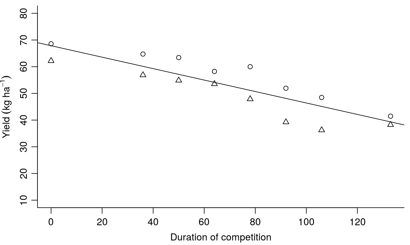
Figure 9.2: The regression model with year as a random effect. Note that in this instance we have one slope and one intercept, and the regression line now is almost in the middle. Note that the fixef(Regression.m2) contains the fixed regressions parameters and the ordinary abline() can be used.
9.1.2 Example 2: Fungicide toxicity
Another example is with a total of six concentration-response experiments evaluating the effect of a fungicide, vinclozolin on luminescence of ovary cells. Vinclozolin is a putative endogenous disruptor and therefore banned in Denmark. The concentration-response curves were run on separate days and it shows that the calibration of the instrument makes the response-curves somewhat different.
vinclozolin <- read.csv("http://rstats4ag.org/data/vinclozolin.csv")
head(vinclozolin)
## conc effect experiment
## 1 0.025 908 10509
## 2 0.050 997 10509
## 3 0.100 744 10509
## 4 0.200 567 10509
## 5 0.390 314 10509
## 6 0.780 325 10509Figure 9.3 shows the individual response curves illustrating the variation in the slope and intercept of the straight lines. However, the variation is kind of erratic because of daily calibration of the machine. Therefore, we consider days a random effect, the variation is intangible. As was the case with the duration of competition we will change the numeric name of each experiment to a factor:
vinclozolin$Experiment <- factor(vinclozolin$experiment)And then run the analysis, but first we illustrate thevariation in data (Figure 9.3).
library(lattice)
xyplot(effect ~ log(conc) | Experiment, data = vinclozolin,
       xlab = "Log( Concentration of Vinclozolin)", ylab = "Luminescence",
       panel = function(x,y)
         {panel.xyplot(x,y)
          panel.lmline(x,y)})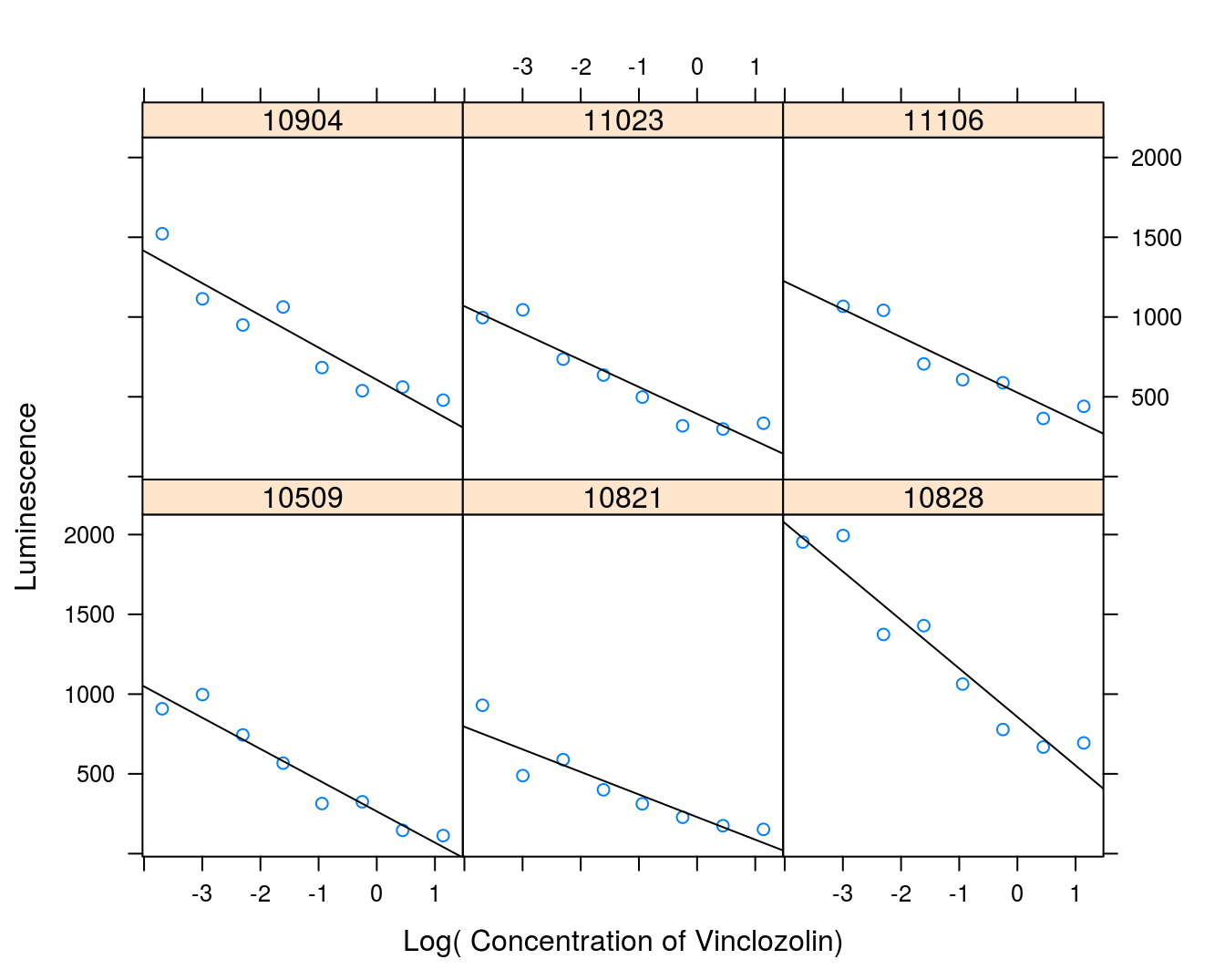
Figure 9.3: Concentration-response curves for ovary cell luminescence on venclozolin.
The procedure to run the mixed regression model is the same as for the sugarbeet example. First we conduct a lack-of-fit test against the most general model - ANOVA.
library(lme4)
vinclo.mixed.ANOVA <- lmer(effect ~ factor(conc) + (1|Experiment),
                           data = vinclozolin, REML = FALSE)
vinclo.mixed.Regression <- lmer(effect ~ log(conc) + (1|Experiment),
                                data = vinclozolin, REML = FALSE)
anova(vinclo.mixed.ANOVA, vinclo.mixed.Regression)
## Data: vinclozolin
## Models:
## vinclo.mixed.Regression: effect ~ log(conc) + (1 | Experiment)
## vinclo.mixed.ANOVA: effect ~ factor(conc) + (1 | Experiment)
## Df AIC BIC logLik deviance Chisq Chi Df Pr(>Chisq)
## vinclo.mixed.Regression 4 627.06 634.46 -309.53 619.06
## vinclo.mixed.ANOVA 10 628.42 646.92 -304.21 608.42 10.64 6 0.1002The test for lack of fit is non-significant so we can assume the relationship is linear, whatever the day. Please note that we only have one replication per regression per day. But the concentrations are the same, so a test for lack of fit is still appropriate.
summary(vinclo.mixed.Regression)## Linear mixed model fit by maximum likelihood ['lmerMod']
## Formula: effect ~ log(conc) + (1 | Experiment)
## Data: vinclozolin
##
## AIC BIC logLik deviance df.resid
## 627.1 634.5 -309.5 619.1 43
##
## Scaled residuals:
## Min 1Q Median 3Q Max
## -1.9356 -0.6270 -0.2354 0.6112 3.0031
##
## Random effects:
## Groups Name Variance Std.Dev.
## Experiment (Intercept) 72092 268.5
## Residual 19987 141.4
## Number of obs: 47, groups: Experiment, 6
##
## Fixed effects:
## Estimate Std. Error t value
## (Intercept) 478.77 112.71 4.248
## log(conc) -199.03 13.31 -14.956
##
## Correlation of Fixed Effects:
## (Intr)
## log(conc) 0.144The variation among experimental days (268) is huge compared with the variation within days (141).
xyplot(effect~log(conc)|experiment, data=vinclozolin,
       xlab="Log( Concentration of Vinclozolin)", ylab="Luminescence",
       panel=function(...)
         {panel.xyplot(...);
          panel.abline(fixef(vinclo.mixed.Regression))})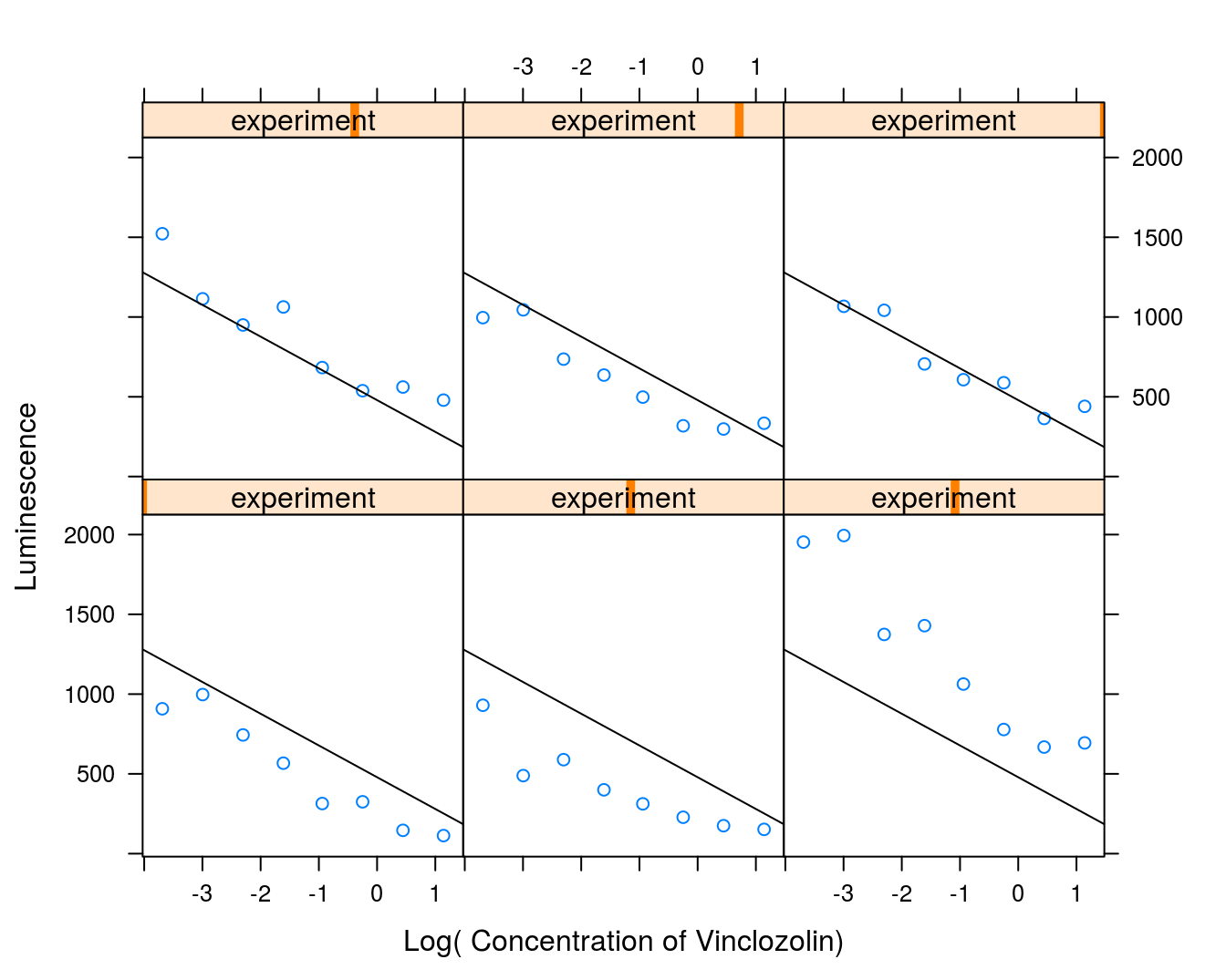
Figure 9.4: Regression lines for all 6 days shown in six panels to give an idea of the variation among days. There appear to be particularly large differences between the responses and the regression lines for the three days in the lower panels.
If we had run an ordinary regression by pooling the six concentration-response curves then we would have gotten the result below.
vinclo.fixed.Regression<-lm(effect ~ log(conc), data = vinclozolin)
summary(vinclo.fixed.Regression)
##
## Call:
## lm(formula = effect ~ log(conc), data = vinclozolin)
##
## Residuals:
## Min 1Q Median 3Q Max
## -584.64 -212.74 -58.83 179.01 920.36
##
## Coefficients:
## Estimate Std. Error t value Pr(>|t|)
## (Intercept) 478.90 58.03 8.253 1.48e-10 ***
## log(conc) -198.53 29.33 -6.768 2.25e-08 ***
## ---
## Signif. codes: 0 '***' 0.001 '**' 0.01 '*' 0.05 '.' 0.1 ' ' 1
##
## Residual standard error: 312.6 on 45 degrees of freedom
## Multiple R-squared: 0.5044, Adjusted R-squared: 0.4934
## F-statistic: 45.8 on 1 and 45 DF, p-value: 2.253e-08The slope and the intercept are almost identical for the two lmer()and lm(). The standard errors for the intercept, though, roughly doubled, 58 for lm() to 113 for lmer(), whereas the slope was more that halved, 13, for the lmer()compared to 29 with lm(). Undoubtedly, the experimental dates improved the precision of the slope. We can compare the fixed and random effects models on these data using Akaike Information Criterion (AIC). For a given set of data, the model with the lowest AIC value is more likely to be the appropriate model.
AIC(vinclo.mixed.Regression, vinclo.fixed.Regression)## df AIC
## vinclo.mixed.Regression 4 627.0628
## vinclo.fixed.Regression 3 677.3501As a gereral rule, differences in AIC values less than 10 indicate two models perform similarly in describing the data. For the vinclozolin data set, the mixed model has and AIC of 627 compared to 677 for the fixed model where the effect of day was not included. This indicates the mixed model is the best fit for these data.