2 Descriptive Statistics
2.1 Calculating group means
One of the most basic exploratory tasks with any data set involves computing the mean, variance, and other descriptive statistics. A previous section has already demonstrated how to obtain many of these statistics from a data set, using the summary(), mean(), and sd() functions. However these functions were used in the context of an entire data set or column from a data set; in most cases it will be more informative to calculate these statistics for groups of data, such as experimental treatments. The tapply() function can be used for this purpose. Summary statistics for the corn irrigation data set were calculated previously using the summary() function. The tapply() function allows us to calculate similar descriptive statistics for groups of data, most commonly for treatments, but also for other logical groups, such as by experimental sites, or years. The tapply() function requires three arguments:
- The data column you want to summarize (response variable)
- The data column you wish to group the data by (treatment or grouping variable)
- The function you want to calculate (mean, standard deviation, maximum, etc.)
The example below will calculate mean yield for each irrigation block (Full irrigation or Limited irrigation).
corn.dat <- read.csv("http://rstats4ag.org/data/irrigcorn.csv")
tapply(corn.dat$Yield.BuA, corn.dat$Irrig, mean)
## Full Limited
## 181.1667 163.2708To specify multiple grouping variables, we use the list() function within the tapply() function:
tapply(corn.dat$Yield.BuA, list(corn.dat$Population.A, corn.dat$Irrig), mean)## Full Limited
## 23000 171.1667 147.3333
## 33000 191.1667 179.20832.2 Calculating other group statistics with tapply
We can use the same syntax to calculate nearly any statistic for the groups by replacing the mean argument with another function, such as max, min, sd etc.
tapply(corn.dat$Yield.BuA, list(corn.dat$Population.A, corn.dat$Irrig), median)## Full Limited
## 23000 171 152.5
## 33000 191 182.5You can also specify other functions or operations. For example, there is no default function in R to calculate the CV, or coefficient of variation. This statistic is commonly used in crop sciences. The CV is simply the standard deviation divided by the mean, and so we can calculate the CV using by storing the output from tapply() into an object that we can call upon later.
popirr.sd   <- tapply(corn.dat$Yield.BuA,
                      list(corn.dat$Population.A, corn.dat$Irrig), sd)
popirr.mean <- tapply(corn.dat$Yield.BuA,
                      list(corn.dat$Population.A, corn.dat$Irrig), mean)
popirr.cv<-popirr.sd/popirr.mean
round(popirr.cv, 3)
## Full Limited
## 23000 0.075 0.102
## 33000 0.052 0.098The round() function simply rounds the result to 3 decimal places to make the output more readable. Alternatively, if the CV is a statistic we will use regularly, it may be worthwhile to write our own function to save keystrokes later on. We can do this using function().
cv <- function(x) {
  xm  <- mean(x)
  xsd <- sd(x)
  xcv <- xsd/xm
  round(xcv, 4)
}
Or, more efficiently:
cv <- function(x) {
  xcv <- round(sd(x) / mean(x), 4)
}
tapply(corn.dat$Yield.BuA, list(corn.dat$Population.A, corn.dat$Irrig), cv)
## Full Limited
## 23000 0.0750 0.1021
## 33000 0.0523 0.0976This approach is desirable if the CV will be used repeatedly. Once the function cv() has been defined, you can call upon it repeatedly with very few keystrokes.
2.3 Using dplyr to summarize data
In addition to using tapply() from base stats R package, there is an excellent package for summarizing data called dplyr. We can get similar information from the corn data set using the dplyr package using the following syntax (explained in more detail below).
library(dplyr)
corn.summary <- corn.dat %>%
  group_by(Population.A, Irrig) %>%
  summarize(N        = length(Yield.BuA),
            AvgYield = round(mean(Yield.BuA),1),
            CV       = cv(Yield.BuA))
corn.summary
## # A tibble: 4 x 5
## # Groups: Population.A [2]
## Population.A Irrig N AvgYield CV
## <int> <fct> <int> <dbl> <dbl>
## 1 23000 Full 24 171. 0.075
## 2 23000 Limited 24 147. 0.102
## 3 33000 Full 24 191. 0.0523
## 4 33000 Limited 24 179. 0.0976We will explain and demonstrate some of the basic uses of dplyr using herbicide resistant weed data from Canada. The following data set was assembled using data from weedscience.org.
resistance<-read.csv("http://rstats4ag.org/data/CanadaResistance2.csv")
resistance<-na.omit(resistance)
head(resistance)
## Province ID SciName Year MOA
## 1 Alberta 1 Stellaria media 1988 ALS inhibitors (B/2)
## 2 Alberta 2 Kochia scoparia 1989 ALS inhibitors (B/2)
## 3 Alberta 3 Avena fatua 1989 Multiple Resistance: 2 Sites of Action
## 6 Alberta 4 Setaria viridis 1989 Microtubule inhibitors (K1/3)
## 7 Alberta 5 Avena fatua 1991 ACCase inhibitors (A/1)
## 8 Alberta 6 Sinapis arvensis 1993 ALS inhibitors (B/2)In the data file, there are instances of multiple resistance (resistance to more than one mode of action). The second line of the code above (na.omit()) removes all lines in the data set that contain NA (which is the default value in R for missing data). This is necessary for this particular example so that instances of multiple resistance are not counted multiple times. We may want to use the information from those rows later on, however, and therefore this method is preferable to deleting the rows from the raw data file.
One of the first things we might like to do is simply count the number of herbicide resistant weed cases by mode of action. We could do this rather quickly using the tapply() function discussed in the previous section: tapply(resistance$ID, resistance$MOA, length). In the code below, we will use the dplyr package to get some interesting information from this data set. First, we can simply count the number of herbicide resistant weeds for each mode of action in the data set. Initially it seems like much more typing compared to using tapply(), but later on it will become clear why this is a potentially more powerful method.
library(dplyr)
bymoa<-group_by(resistance, MOA)
moatotal<-summarize(bymoa, total=length(ID))
print(moatotal)
In the code above, we are loading the dplyr package, then using two functions from that package. The group_by() function will provide the information on how the data are grouped. In this case, we want to group the data by MOA. We can then use the the summarize() function to calculate means, counts, sums, or any other operation on the data. Above, we used the length() function to count the unique instances of the ID variable for each mode of action. Storing each step with the <- operator can be a little cumbersome, especially if we will not need to use the intermediary steps again. The dplyr package uses the %>% operator to string together several steps. The code below will result in the same summary as above, with fewer keystrokes, and without storing the intermediary grouping as a separate object. The first line provides the name of the data set (resistance) followed by the %>% operator. This tells R to expect a function on the next line from the dplyr package. The second line groups the resistance data set by MOA, and the third line summarizes the data by calculating the length of the ID variable for each level of the grouping factor. Effectively, this counts each instance of resistance. The last line prints out the resulting data frame.
moatotal <- resistance %>%
  group_by(MOA) %>%
  summarize(total=length(ID))
print(moatotal)
## # A tibble: 13 x 2
## MOA total
## <fct> <int>
## 1 ACCase inhibitors (A/1) 9
## 2 ALS inhibitors (B/2) 42
## 3 EPSP synthase inhibitors (G/9) 2
## 4 Lipid Inhibitors (thiocarbamates) (N/8) 2
## 5 Microtubule inhibitors (K1/3) 3
## 6 "Multiple Resistance: 2 Sites of Action " 12
## 7 "Multiple Resistance: 3 Sites of Action " 3
## 8 "Multiple Resistance: 4 Sites of Action " 1
## 9 Photosystem II inhibitors (C1/5) 12
## 10 PSI Electron Diverter (D/22) 3
## 11 PSII inhibitors (Nitriles) (C3/6) 2
## 12 PSII inhibitor (Ureas and amides) (C2/7) 3
## 13 Synthetic Auxins (O/4) 3The real power and elegance of the dplyr package becomes apparent once we begin using multiple groupings, and creating new variables. Below, we generate totals for each mode of action again, but also by year of listing by using the group_by() and sumarize() functions.
totals<-resistance %>%
  group_by(Year, MOA) %>%
  summarize(total = length(ID))
head(totals)
## # A tibble: 6 x 3
## # Groups: Year [6]
## Year MOA total
## <int> <fct> <int>
## 1 1957 Synthetic Auxins (O/4) 1
## 2 1973 Photosystem II inhibitors (C1/5) 1
## 3 1976 Photosystem II inhibitors (C1/5) 2
## 4 1977 Photosystem II inhibitors (C1/5) 3
## 5 1980 Photosystem II inhibitors (C1/5) 1
## 6 1981 Photosystem II inhibitors (C1/5) 3We can then create a new variable using the mutate() function; we will add a cumulative total of herbicide resistance cases over time, while retaining information about mode of action by first ungrouping the data, then using mutate to calculate the cumulative total using the cumsum() from the default stats package.
totals <- resistance %>%
  group_by(Year, MOA) %>%
  summarize(total = length(ID)) %>%
  ungroup() %>%
  mutate(cumulative = cumsum(total))

head(totals)
## # A tibble: 6 x 4
## Year MOA total cumulative
## <int> <fct> <int> <int>
## 1 1957 Synthetic Auxins (O/4) 1 1
## 2 1973 Photosystem II inhibitors (C1/5) 1 2
## 3 1976 Photosystem II inhibitors (C1/5) 2 4
## 4 1977 Photosystem II inhibitors (C1/5) 3 7
## 5 1980 Photosystem II inhibitors (C1/5) 1 8
## 6 1981 Photosystem II inhibitors (C1/5) 3 11tail(totals)## # A tibble: 6 x 4
## Year MOA total cumulative
## <int> <fct> <int> <int>
## 1 2010 EPSP synthase inhibitors (G/9) 1 88
## 2 2011 ACCase inhibitors (A/1) 1 89
## 3 2011 ALS inhibitors (B/2) 2 91
## 4 2011 "Multiple Resistance: 2 Sites of Action " 2 93
## 5 2012 ALS inhibitors (B/2) 1 94
## 6 2012 "Multiple Resistance: 2 Sites of Action " 3 97Based on the final row of data, there are 97 unique cases of herbicide resistance in this data set. And now, we can use the new data frame generated by dplyr to make a plot of cumulative herbicide resistance cases over time, coded by herbicide mode of action. The specifics of plotting are discussed in the Data Visualization section.
par(bg=gray(0.95), mar=c(4.5,4.5,0.8,0.8), mgp=c(2,.7,0))
plot(cumulative~Year, col=as.numeric(MOA), pch=as.numeric(MOA),
     data=totals, ylab="Herbicide Resistant Weed Cases in Canada")
legend("topleft", legend=unique(totals$MOA),
       col=as.numeric(unique(totals$MOA)),
       pch=as.numeric(unique(totals$MOA)))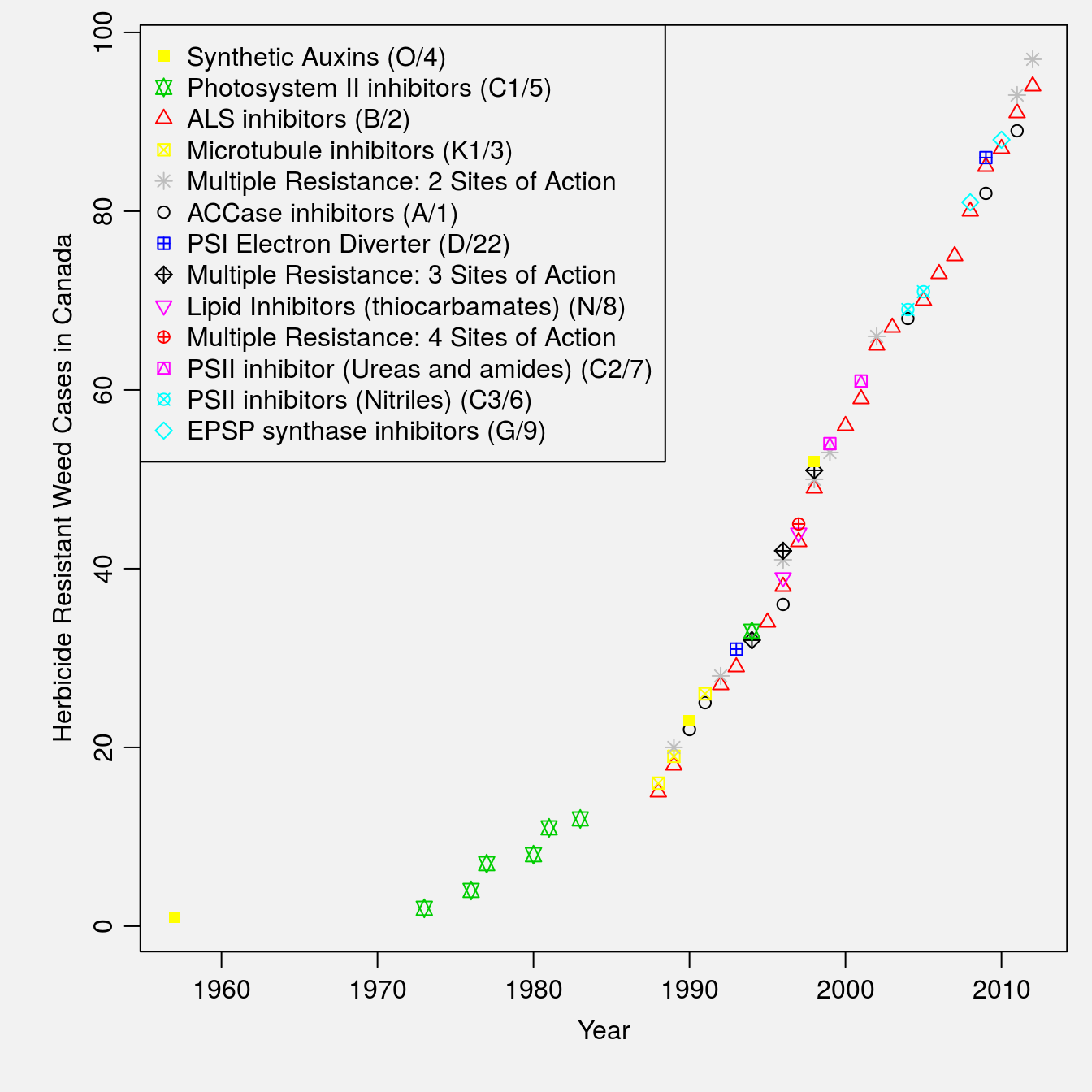
Figure 2.1: Cumulative number of herbicide resistant weed cases in Canada over time.
We can also use dplyr to look at other grouping, including by province or weed species, and then use the subset() function to print out only one group. In the below example, we will calculate totals for each province by weed species, but print out only the cases of herbicide resistant weeds from Saskatchewan.
provspec <- resistance %>%
  group_by(Province, SciName) %>%
  summarize(total=length(ID))
subset(provspec, Province=="Saskatchewan")
## # A tibble: 12 x 3
## # Groups: Province [1]
## Province SciName total
## <fct> <fct> <int>
## 1 Saskatchewan Amaranthus retroflexus 1
## 2 Saskatchewan Avena fatua 4
## 3 Saskatchewan Capsella bursa-pastoris 1
## 4 Saskatchewan Chenopodium album 1
## 5 Saskatchewan Galium spurium 1
## 6 Saskatchewan Kochia scoparia 2
## 7 Saskatchewan Lolium persicum 1
## 8 Saskatchewan Salsola tragus 1
## 9 Saskatchewan Setaria viridis 3
## 10 Saskatchewan Sinapis arvensis 1
## 11 Saskatchewan Stellaria media 1
## 12 Saskatchewan Thlaspi arvense 1