5 Analysis of Variance (ANOVA)
5.1 One-Way Analysis of Variance
Some of the most often used experimental designs in weed science include completely randomized designs (CRD) and randomized complete block designs (RCBD). These experiments are typically analyzed using analysis of variance (ANOVA). The one-way ANOVA is used to determine the effect of a single factor (with at least three levels) on a response variable. Where only two levels of a single factor are of interest, the t.test() function will be more appropriate. There are several ways to conduct an ANOVA in the base R package. The aov() function requires a response variable and the explanatory variable separated with the ~ symbol. It is important when using the aov() function that your data are balanced, with no missing values. For data sets with missing values or unbalanced designs, please see the section on mixed effects models.
The “FlumiBeans” data set is from a herbicide trial conducted in Wyoming during three different years (2009 through 2011). Five different herbicide treatments were applied, plus nontreated and handweeded controls for a total of seven treatments. The study was a randomized complete block design (RCBD) each year. There were 3 replicates in 2009, but 4 replicates in subsequent years. The response variable in this data set is dry bean (Phaseolus vulgaris) density 4 weeks after planting expressend in plants per acre.
read.csv("http://rstats4ag.org/data/FlumiBeans.csv")->bean.dat
bean.dat$population.4wk <- bean.dat$population.4wk * 2.47 # Convert to SI units
summary(bean.dat)
## year treatment block population.4wk
## Min. :2009 EPTC + ethafluralin :11 Min. :1.000 Min. : 17216
## 1st Qu.:2009 flumioxazin + ethafluralin :11 1st Qu.:1.000 1st Qu.: 51648
## Median :2010 flumioxazin + pendimethalin:11 Median :2.000 Median : 94683
## Mean :2010 flumioxazin + trifluralin :11 Mean :2.364 Mean : 87836
## 3rd Qu.:2011 Handweeded :11 3rd Qu.:3.000 3rd Qu.:114052
## Max. :2011 imazamox + bentazon :11 Max. :4.000 Max. :163541
## Nontreated :11It is important to note that some of our factor variables have been expressed in the .csv file as numbers (e.g. ‘year’ and ‘block’), and consequently, R has recognized these factors as numeric variables. It is important for our ANOVA that these variables be included as factors, and not as numeric variables. We can tell R to view these variables as factors by re-naming them using the as.factor() function.
bean.dat$year<-as.factor(bean.dat$year)
bean.dat$block<-as.factor(bean.dat$block)
summary(bean.dat)
## year treatment block population.4wk
## 2009:21 EPTC + ethafluralin :11 1:21 Min. : 17216
## 2010:28 flumioxazin + ethafluralin :11 2:21 1st Qu.: 51648
## 2011:28 flumioxazin + pendimethalin:11 3:21 Median : 94683
## flumioxazin + trifluralin :11 4:14 Mean : 87836
## Handweeded :11 3rd Qu.:114052
## imazamox + bentazon :11 Max. :163541
## Nontreated :11Notice the difference for the ‘year’ and ‘block’ variables in the summary() results before and after renaming. For this analysis, we want to look at a One-Way analysis of variance, and so we will focus on the data from only one year. We can subset the data by year, and call this subsetted data bean.09.
bean.09<-subset(bean.dat, year==2009)We will then use the aov() function to generate the One-way ANOVA to see if herbicide treatment had an effect on dry bean population (expressed in plants per hectare) in 2009.
aov(population.4wk ~ block+treatment, data=bean.09)->b09.aov5.1.1 Checking ANOVA assumptions
ANOVA assumes (1) errors are normally distributed, (2) variances are homogeneous, and (3) observations are independent of each other. ANOVA is fairly robust to violations of the normality assumption, and thus it typically requires a rather severe violation before remedial measures are warranted. However, it is still wise to check the normality assumption prior to interpreting the ANOVA results. Three methods are provided to check normality of the response variable of interest: the Shapiro-Wilks test, a stem and leaf plot, and a Normal Q-Q plot. The model residuals are automatically stored within the ANOVA model produced with the aov() function, and thus we can call upon the model to view and test the residuals for normality. We can get the residuals by using the resid() function, or by appending $resid onto the model fit. resid(b09.aov) and b09.aov$resid will provide the same result.
shapiro.test(b09.aov$resid)##
## Shapiro-Wilk normality test
##
## data: b09.aov$resid
## W = 0.9718, p-value = 0.7726stem(b09.aov$resid)##
## The decimal point is 4 digit(s) to the right of the |
##
## -2 | 690
## -0 | 88607431
## 0 | 222599
## 2 | 2787par(mar=c(3.2,3.2,2,0.5), mgp=c(2,.7,0))
qqnorm(b09.aov$resid)
qqline(b09.aov$resid)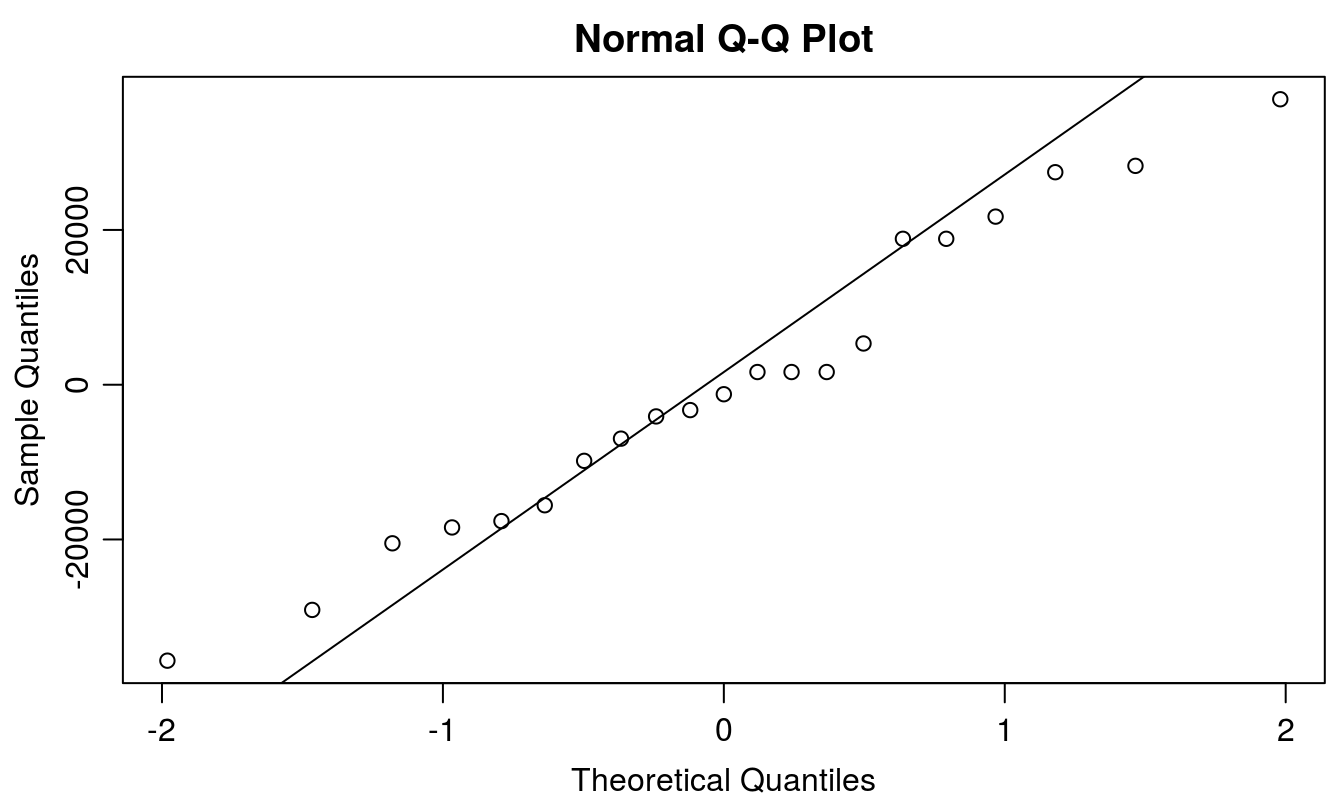
Figure 5.1: Normal Q-Q plot to check the assumption of normal distribution of residuals.
It appears that the residuals in this case are at least close to normally distributed. The most common next step if residuals are not normally distributed would be to attempt a transformation. However, it is worth noting that there are other, more modern methods to deal with non-normality that should be strongly considered.
The next assumption to test is homogeneity of variance. Formal tests for homogeneity of variance include the Bartlett (parametric) and Fligner-Killeen (non-parametric) tests. These tests can be used in conjunction with box plots to determine the level of heterogeneity of variance between treatments.
bartlett.test(bean.09$population.4wk, bean.09$treatment)##
## Bartlett test of homogeneity of variances
##
## data: bean.09$population.4wk and bean.09$treatment
## Bartlett's K-squared = 3.7865, df = 6, p-value = 0.7055fligner.test(bean.09$population.4wk, bean.09$treatment)##
## Fligner-Killeen test of homogeneity of variances
##
## data: bean.09$population.4wk and bean.09$treatment
## Fligner-Killeen:med chi-squared = 3.2494, df = 6, p-value = 0.777Formal tests do not indicate a problem (p>0.7), and box plots (Figure 5.2) indicate that things are reasonable similar. Perhaps the handweeded and EPTC + ethalfluralin treatments have less variability than the others, but differences are not too dramatic, especially considering there were only 3 replicates per treatment in 2009.
par(mar=c(4.2,12,0.5,1.5), mgp=c(2,.7,0))
boxplot(bean.09$population.4wk/1000 ~ bean.09$treatment, horizontal=T,
        las=1, xlab="Bean plants per hectare (thousands)")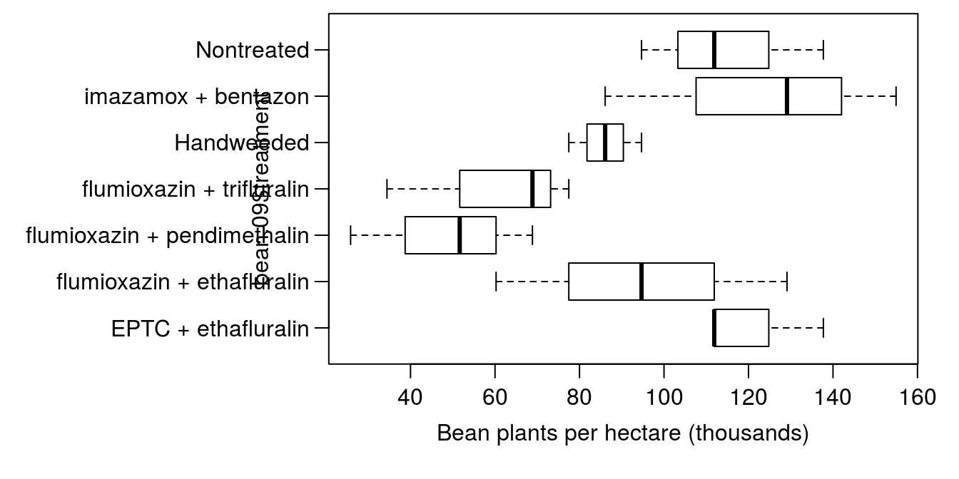
Figure 5.2: Boxplots showing the effect of weed control treatment on dry edible bean plants per hectare.
Simply plotting the aov fit in R [e.g. Figure 5.3] will provide a series of diagnostic plots as well. The first two plots are the residuals vs fitted values, and the Normal Q-Q plot, which can be plotted at the same time with the following code:
par(mar=c(4.2,4.2,2.2,1), mfrow=c(1,2), mgp=c(2,.7,0))
plot(b09.aov, which=1:2)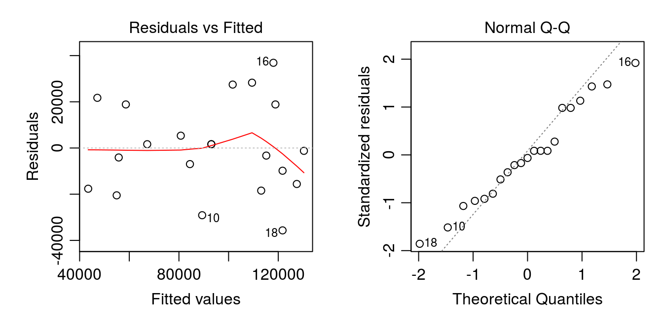
Figure 5.3: Model diagnostic plots for the dry edible bean ANOVA model.
Since neither the normality nor homogeneity of variance assumptions were dramatically violated, and ANOVA is fairly robust to violations of these assumptions, it seems safe to proceed with interpretation of the ANOVA results. The third assumption (independence of observations) is not something we will test statistically; it is up to the researcher to ensure that they are collecting data in a way that does not violate this assumption.
Finally, after the assumptions have been checked, and remedial measures taken if necessary, we will want to know whether there is a significant effect of herbicide treatment on dry bean population density. Once again, we can use the summary() function along with the stored model to obtain this information. The resulting ANOVA table indicates that we have pretty strong evidence that there are differences in dry bean plants per acre due to herbicide treatment (p = 0.019).
summary(b09.aov)## Df Sum Sq Mean Sq F value Pr(>F)
## block 2 5.574e+08 2.787e+08 0.432 0.6589
## treatment 6 1.569e+10 2.615e+09 4.055 0.0188 *
## Residuals 12 7.740e+09 6.450e+08
## ---
## Signif. codes: 0 '***' 0.001 '**' 0.01 '*' 0.05 '.' 0.1 ' ' 15.1.2 Mean Separation - agricolae package
The agricolae package has several functions for mean separation, including the LSD.test() function that will compare means using Fisher’s LSD. The LSD.test computes a lot of useful information that can be extracted for later use. You can use the str(bean.lsd) function to learn more about what is available. Below, we will look at the $group section which gives the treatment means and mean separation, and the $statistics section which provides the LSD value (among other things).
library(agricolae)
bean.lsd <- LSD.test(b09.aov, trt="treatment")
bean.lsd$group
## population.4wk groups
## imazamox + bentazon 123373.21 a
## EPTC + ethafluralin 120503.89 a
## Nontreated 114766.08 a
## flumioxazin + ethafluralin 94682.51 ab
## Handweeded 86074.56 abc
## flumioxazin + trifluralin 60251.53 bc
## flumioxazin + pendimethalin 48775.09 cbean.lsd$statistics## MSerror Df Mean CV t.value LSD
## 645034519 12 92632.41 27.41754 2.178813 45182.03To get standard deviations and confidence limits, we could type bean.lsd$means. The agricolae package can also calculate Tukey’s HSD using the HSD.test() function. The syntax above is the same, simply changing LSD.test to HSD.test.
5.1.3 Mean Separation - multcomp package
The multcomp package is also useful for separating means, and has the advantage that it can be used for linear, nonlinear, and mixed effects models.
library(multcomp)
b09.tukey <- summary(glht(b09.aov, linfct=mcp(treatment = "Tukey")))
b09.tukey # prints out all pairwise comparisons
cld(b09.tukey) # prints out the compact letter display (cld)
5.2 Multi-Factor ANOVA
We’ll now look at the second and third year of the study, beginning by subsetting the data to include only these years.
bean2.dat<-subset(bean.dat, year==2010 | year==2011)
summary(bean2.dat)
## year treatment block population.4wk
## 2009: 0 EPTC + ethafluralin :8 1:14 Min. : 17216
## 2010:28 flumioxazin + ethafluralin :8 2:14 1st Qu.: 51645
## 2011:28 flumioxazin + pendimethalin:8 3:14 Median : 95761
## flumioxazin + trifluralin :8 4:14 Mean : 86038
## Handweeded :8 3rd Qu.:115665
## imazamox + bentazon :8 Max. :163541
## Nontreated :8We’ll now incorporate year as a fixed effect in the analysis. We’re going to exclude the 2009 data because it does not have the same number of replicates as the other two years of data. The aov() function is not appropriate for unbalanced data. We will look at how to best handle this in a later section using mixed effects. We’re also going to incorporate the blocking design into the model using the Error() argument. Blocking was used in each year of the field study (in a randomized complete block design). Because the trial was located in a different field each year, there is no reason to think that block 1 would result in a similar impact from one year to the next. Therefore, the effect of block is nested within year. We can specify this structure in the aov() function by using the / operator.
bean2.aov<-aov(population.4wk ~ year*treatment + Error(year/block), data=bean2.dat)
summary(bean2.aov)
##
## Error: year
## Df Sum Sq Mean Sq
## year 1 5.46e+09 5.46e+09
##
## Error: year:block
## Df Sum Sq Mean Sq F value Pr(>F)
## Residuals 6 1.363e+09 227216916
##
## Error: Within
## Df Sum Sq Mean Sq F value Pr(>F)
## treatment 6 6.588e+10 1.098e+10 51.925 2.91e-16 ***
## year:treatment 6 5.422e+09 9.036e+08 4.273 0.00238 **
## Residuals 36 7.612e+09 2.114e+08
## ---
## Signif. codes: 0 '***' 0.001 '**' 0.01 '*' 0.05 '.' 0.1 ' ' 1Adding the Error term into the model results in 3 separate sections of the ANOVA table, corresponding to the three separate error terms: year, year:block, and within. In this case no F or P-values are calculated for the year effect. We could do that manually by dividing the Mean Square for year by the Mean Square for year:block, but it is clear just by looking at the numbers that the F value will be quite high (greater than 23, in fact). However, if we want aov() to calculate the P-value for us, we can specify the year*block error term by creating a new variable that contains the combined information. We will do this below using the with() function.
bean2.dat$yrblock  <- with(bean2.dat, factor(year):factor(block))
bean2.aov2<-aov(population.4wk ~ year*treatment + Error(yrblock), data=bean2.dat)
summary(bean2.aov2)
##
## Error: yrblock
## Df Sum Sq Mean Sq F value Pr(>F)
## year 1 5.460e+09 5.460e+09 24.03 0.00271 **
## Residuals 6 1.363e+09 2.272e+08
## ---
## Signif. codes: 0 '***' 0.001 '**' 0.01 '*' 0.05 '.' 0.1 ' ' 1
##
## Error: Within
## Df Sum Sq Mean Sq F value Pr(>F)
## treatment 6 6.588e+10 1.098e+10 51.925 2.91e-16 ***
## year:treatment 6 5.422e+09 9.036e+08 4.273 0.00238 **
## Residuals 36 7.612e+09 2.114e+08
## ---
## Signif. codes: 0 '***' 0.001 '**' 0.01 '*' 0.05 '.' 0.1 ' ' 1The Mean Square for year and the year:block interaction are the same as before, as expected, but now the F and P-values are provided. However, this is not as important in this case, as there is a significant year by treatment interaction effect, making the main effect of year less interesting.
5.2.1 Mean Separation
Due to the different error terms, getting mean separation from the LSD.test() function in this case is not as straightforward as with only one factor. It can still be done by specifying the response, treatment, error degrees of freedom, and mean square error manually.
bean2.lsd<-LSD.test(bean2.dat$population.4wk,
                    with(bean2.dat, year:treatment),
                    36, 2.11e+08)
bean2.lsd$groups
## bean2.dat$population.4wk groups
## 2010:imazamox + bentazon 142023.15 a
## 2010:EPTC + ethafluralin 139871.16 a
## 2010:Handweeded 124807.87 ab
## 2010:Nontreated 124807.87 ab
## 2011:Handweeded 104369.23 bc
## 2011:Nontreated 97375.43 c
## 2011:imazamox + bentazon 95761.28 c
## 2011:EPTC + ethafluralin 94147.76 c
## 2011:flumioxazin + trifluralin 57026.74 d
## 2010:flumioxazin + trifluralin 51644.61 de
## 2010:flumioxazin + pendimethalin 49493.24 de
## 2011:flumioxazin + pendimethalin 48956.64 de
## 2010:flumioxazin + ethafluralin 38733.92 de
## 2011:flumioxazin + ethafluralin 35506.87 eIt seems there is general trend for treatments containing flumioxazin to have fewer bean plants. But having the different years mixed together makes it difficult to see, so an alternative approach would be to simply calculate the means using tapply() and print out the LSD value.
round(tapply(bean2.dat$population.4wk,
             list(bean2.dat$treatment, bean2.dat$year), mean), -3)
## 2009 2010 2011
## EPTC + ethafluralin NA 140000 94000
## flumioxazin + ethafluralin NA 39000 36000
## flumioxazin + pendimethalin NA 49000 49000
## flumioxazin + trifluralin NA 52000 57000
## Handweeded NA 125000 104000
## imazamox + bentazon NA 142000 96000
## Nontreated NA 125000 97000bean2.lsd$statistics## MSerror Df Mean CV t.value LSD
## 2.11e+08 36 86037.55 16.88314 2.028094 20831.2Looking at the data in this way makes it appear that the year interaction was due to a higher bean population in 2010 compared to 2011 for most treatments. However, the flumioxazin treatments had similar bean populations in both years, much reduced compared to the nontreated or handweeded control treatments. The LSD value of 0 allows us to compare the same treatment between years, or compare between treatments within a year.